Estimation

amorem’s estimation surface has these layers:

Case-control sampling turns a raw event log into a stratified table that survival / GLM tools can fit directly (sample_non_events(); widen_case_control() reshapes it to the wide case-1-control form).
rem() — the unified fitter for (already preprocessed) case-control data: a conditional-logit backend for case-k-control designs and a gam backend for case-1-control, with linear / TV / NL / TVNL effects and summary() / coef() / plot() methods.
compare_models* helpers evaluate a list of candidate specifications on a single sample and return a tidy AIC table (superseded by rem(), still supported).
Goodness-of-fit tests check whether the selected fit is actually adequate.

Every numerical output below is produced by paper/wiki/experiments/est_demo.R, which is re-run on every release of the wiki.

Case-control sampling

The partial likelihood for a relational event model factors over events, with each factor a ratio between the firing dyad’s rate and the sum of rates over the risk set at that moment. The case-control approximation replaces the full risk set sum with an unbiased Horvitz-Thompson estimate that uses n_controls sampled non-firing dyads per case.

Throughout this page we use the bundled classroom_events log — any event log with time, sender, receiver columns will do.

library(amorem)
data(classroom_events)

cc <- sample_non_events(classroom_events,
                        n_controls = 1,
                        scope      = "all",
                        mode       = "one")

scope selects which non-firing dyads form the candidate pool ("all", "appearance", or "citation"); mode selects the sampling design ("one" matched-set or "two" permuted).

Risk-set exclusions. Two further controls keep ineligible dyads out of the candidate pool. exclude_pairs is a two-column (sender, receiver) table of dyads that are structurally ineligible — e.g. an alien species’ native range, forbidden transitions, same-department pairs — and are never sampled as controls. And under risk = "remove", a dyad firing at the focal event’s own timestamp is now treated as a concurrent event (not a valid non-event at that instant) and excluded from its control pool:

cc <- sample_non_events(event_log,
                        scope         = "all",
                        mode          = "two",
                        risk          = "remove",          # drops past + concurrent
                        exclude_pairs = native[, c("species", "region")])

For n_controls = 1 the estimator is a no-intercept binomial GLM on case-minus-control differences (asymptotically equivalent to the case-control partial likelihood for 1:1 matched designs). For n_controls > 1 it is a stratified Cox model via survival::coxph (the same machinery survival::clogit calls internally). AIC values are comparable across specifications that share a case-control draw.

To compute endogenous covariates for the sampled non-events without letting them enter the event history, pass the true event log as history_log to endogenous_features() — only rows present in history_log update the running network state.

For set-valued covariates, the "sender_receivers_set" statistic returns a list-column: for each row, the set of receivers the row’s sender has reached before it (e.g. the regions a species has already invaded). It honours history_log too, so it is correct for non-events. Downstream, you join it to an external lookup to build the actual covariate:

feats <- endogenous_features(cc, stats = "sender_receivers_set",
                                     history_log = event_log)
feats$invaded <- Map(setdiff, feats$sender_receivers_set, native_range(feats$sender))
feats$dt      <- mapply(min_climatic_diff, feats$invaded, feats$receiver, feats$time)

`rem()` · unified fitter for preprocessed data

When the covariates have already been computed — e.g. by eventnet or by endogenous_features() — rem() fits the model directly from the case-control table, decoupling fitting from feature computation. It has three backends:

method = "clogit" — conditional logistic regression on a case-k-control design (survival::clogit). Strata come from stratum, or are derived as cumsum(case == 1) for the eventnet blocked layout. Linear terms only.
method = "nn" — a neural conditional-logistic model on the same case-k-control design as clogit: a multilayer perceptron scores every candidate and the loss is the softmax over each risk set, i.e. exactly the conditional partial likelihood with a learned nonlinear intensity in place of the linear predictor. Prediction-oriented — no coefficient table; it earns its keep when effects interact or bend in ways an additive model cannot capture. Pure R, no extra dependencies.
method = "gam" — degenerate logistic regression on a case-1-control design (mgcv::gam), supporting smooth effects. In the formula a bare name is a linear effect; wrap it as tv(x), nl(x) or tvnl(x) for a time-varying, non-linear, or time-varying-non-linear smooth, or re(x) for an actor (or other grouping) random effect — s(cbind(x_ev, x_nv), by = c(1, -1), bs = "re"), the matched event/control random effect (identified when the event and control differ on x).

# case-20-control conditional logit (e.g. an eventnet-preprocessed log)
fit20 <- rem(IS_OBSERVED ~ individual.activity + dyadic.activity,
             data = lesmis, method = "clogit", stratum = "EVENT_INTERVAL")
coef(fit20); summary(fit20)

# case-1-control degenerate logistic with a non-linear effect
w    <- widen_case_control(lesmis, stratum = "EVENT_INTERVAL")
fit1 <- rem(~ nl(dyadic.activity), data = w, method = "gam")
plot(fit1)            # the fitted smooth panel

# neural conditional logit on the same long case-control log
fitnn <- rem(IS_OBSERVED ~ individual.activity + dyadic.activity,
             data = lesmis, method = "nn", stratum = "EVENT_INTERVAL",
             nn = nn_control(hidden = c(16, 8), epochs = 300, seed = 1))
summary(fitnn)               # architecture, in-sample & held-out concordance
plot(fitnn$fit, type = "pdp")  # learned per-feature effect curves

The nn backend is trained full-batch with Adam, early-stops on a held-out fraction of strata (nn_control(validation = , patience = )), and standardizes features internally. logLik() returns the partial likelihood at the trained network, so AIC()-style comparisons against clogit fits are possible (with the usual caveats about effective degrees of freedom for neural networks). Because it shares the case-control machinery, everything upstream — sample_non_events(), feature engineering, stratum handling — is identical to the other backends.

widen_case_control() reshapes a long case-(k-)control log into the wide <cov>_ev / <cov>_nv / d_<cov> form the gam backend expects (one row per case). Undirected logs (set-valued senders, no receiver column) are supported throughout. Column resolution follows the eventnet conventions (x, d_x, x_ev/x_nv, transform_x_*, transformed_time).

rem() supersedes compare_models() / compare_models_smooth() / compare_models_global(), which remain available and are documented below.

`compare_models()` · linear AIC table

A single call evaluates a list of candidate specifications on a shared case-control sample:

data(classroom_events)
compare_models(
  classroom_events,
  models = list(
    count       = c("reciprocity_count", "transitivity_count"),
    continuous  = c("reciprocity_time_recent",
                    "transitivity_time_recent"),
    interrupted = c("reciprocity_time_recent_interrupted",
                    "transitivity_time_recent_interrupted")),
  n_controls = 1, seed = 11)
#>         model n_terms n_obs   log_lik      AIC delta_AIC
#> 1       count       2   691 -305.5233 615.0466     0.000
#> 2  continuous       2   691 -421.1231 846.2462   231.200
#> 3 interrupted       2   691 -439.6904 883.3809   268.334

Runtime: 0.3 s.

compare_models AIC

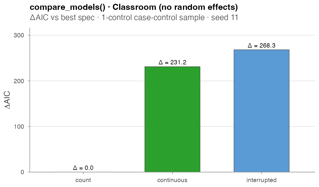
Read this with caution. Without an actor-heterogeneity correction, *_count statistics absorb sender / receiver activity differences directly, so a spec that should encode “how recently did this dyad fire?” reduces to “how active is this sender?”. The naive count win is a well-known artefact. Adding a sender frailty term flips the ranking to continuous by ΔAIC ≈ 6, recovering Table 3 of Juozaitienė & Wit (2024) — see Real-data analysis for the corrected fit.

Argument	Meaning
`event_log`	data frame with `sender`, `receiver`, `time`
`models`	named list of character vectors of stat names
`n_controls`	controls per case (`1`: GLM; `> 1`: stratified Cox)
`scope`, `mode`	passed to `sample_non_events()`
`random_effects`	`"sender"` or `"receiver"` — see below
`half_life`	required when any spec uses an exp-decay stat
`seed`	for the shared case-control draw
`keep_fits`	if `TRUE`, attach the fitted models as `attr(result, "fits")`

All three compare_models*() helpers accept keep_fits = TRUE, which attaches the fitted model objects — one per spec, named by model — as attr(result, "fits"), so an individual fit can be pulled out for plotting its estimated effects:

res <- compare_models_smooth(event_log, models, keep_fits = TRUE)
plot(attr(res, "fits")[["nl"]])     # the chosen spec's smooth panel

Actor random effects

compare_models() accepts random_effects = "sender" or "receiver" (requires n_controls > 1). Internally this injects a Gamma survival::frailty() term on the requested actor axis into the stratified Cox fit, matching the convention in Juozaitienė & Wit (2024).

Two-axis frailty (random_effects = c("sender", "receiver")) is supported via coxme::coxme and is the right tool when both sender and receiver heterogeneity matter; one coxme fit per spec typically runs in seconds to a minute on Classroom-sized data. Requires the coxme package (Suggests).

`compare_models_smooth()` · TV / NL / TVNL effects

Where compare_models() fits a single coefficient per statistic, compare_models_smooth() lets each statistic take one of four effect types: linear, tv (time-varying), nl (non-linear in the covariate), or tvnl (jointly time-varying non-linear via a tensor product smooth). Implementation follows Boschi, Lerner & Wit (2025) Section 3.3:

compare_models_smooth(
  classroom_events,
  models = list(
    linear = c(reciprocity_time_recent  = "linear",
               transitivity_time_recent = "linear"),
    nl    = c(reciprocity_time_recent  = "nl",
               transitivity_time_recent = "nl"),
    tv    = c(reciprocity_time_recent  = "tv",
               transitivity_time_recent = "tv")),
  seed = 11, k = 5)
#>    model n_terms n_obs   log_lik      AIC delta_AIC
#> 1    nl       2   691 -418.3044 845.6569     0.000
#> 2 linear       2   691 -421.1231 846.2462     0.589
#> 3    tv       2   691 -420.7474 849.6835     4.027

Runtime: 1.9 s.

compare_models_smooth AIC

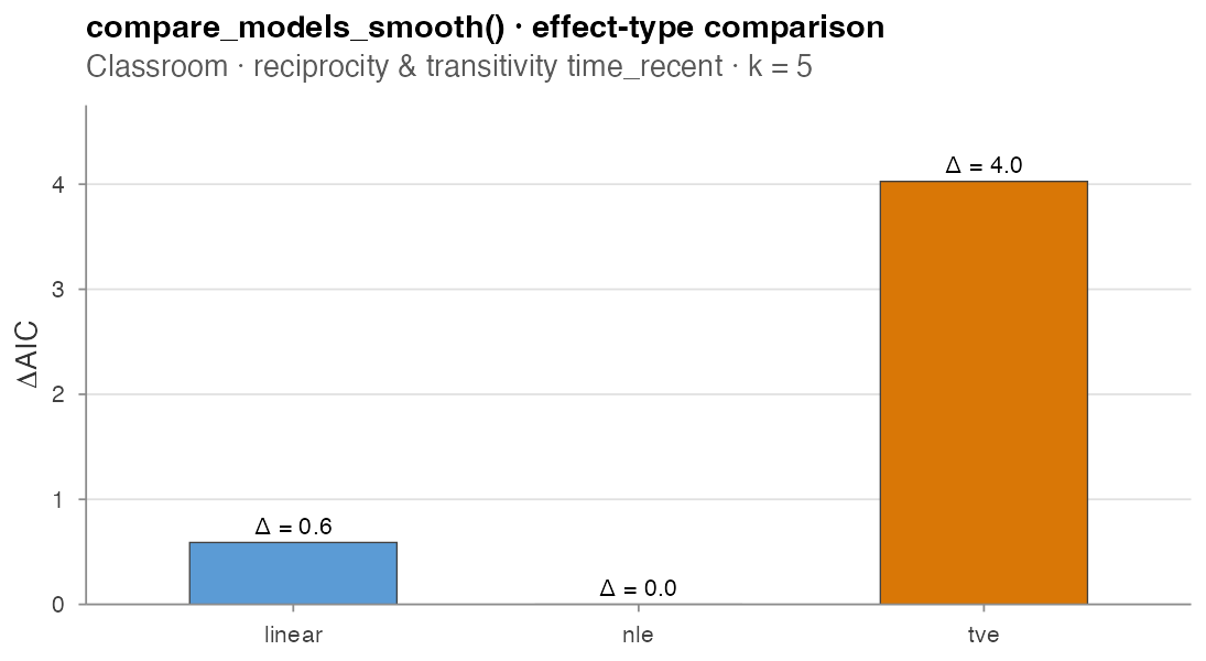
The three specs are within 4 AIC points of each other on the recency-time terms — there is no signal in this dataset that a time-varying or non-linear effect adds value over the linear baseline. The case-vs-control matrix design behind these fits is described in detail at the bottom of this section.

Effect	Smooth term
`linear`	single column `d_stat = case − control`
`tv`	`s(.time, by = d_stat)`
`nl`	`s(stat_mat, by = I_mat)` with `stat_mat = cbind(case, control)`, `I_mat = cbind(1, -1)`
`tvnl`	`te(time_mat, stat_mat, by = I_mat)`

The model is fit by mgcv::gam(method = "REML") with the degenerate logistic likelihood from Boschi et al. equation 8. AIC values are directly comparable across specs because every fit shares the same case-control sample.

`compare_models_global()` · global covariate effects

A global covariate varies in time but is constant across all interacting pairs at any given instant — temperature, time-of-day, the residual baseline hazard g_0(t). Standard case-control partial likelihood structurally cannot identify a global effect because it cancels in the focal-vs-control rate ratio (both pairs are evaluated at the same time). The fix of Lembo, Juozaitienė, Vinciotti & Wit (2025) is a random per-dyad time shift H_sr ~ Exp(rate), so the focal event and the sampled non-event are evaluated at different times. With one non-event per event the partial likelihood collapses to a degenerate logistic GAM that mgcv fits directly:

g <- data.frame(time        = seq(0, max(classroom_events$time), length = 50),
                temperature = sin(seq(0, 2 * pi, length = 50)))
compare_models_global(
  classroom_events,
  models = list(
    dyadic_only = c(reciprocity_count = "linear",
                    transitivity_count = "linear"),
    with_global = c(reciprocity_count = "linear",
                    temperature       = "global_smooth")),
  global_covariates = g, seed = 11, k = 5)

Effect type	Smooth	Use
`global_smooth`	`s(x_global)`	generic global covariate
`global_cyclic`	`s(x_global, bs = "cc")`	periodic axes (time-of-day)
`global_time`	smooth on time itself	recovers residual `g_0(t)`

shift_scale (default 1) multiplies the mean inter-event time used to set the exponential rate of H_sr. Larger values widen the shifts and improve identifiability of slow global signals at the cost of bias under fast-varying g_0. The global_time spec can produce a degenerate fit on small / uninformative data — when this happens the result is NA rather than a hard error.

Recency preprocessing

transform_recency(delta, half_life = NULL, reference = NULL) maps non-negative inter-event time gaps to bounded weights via exp(-delta / (2 m)), with m the median of the supplied (or reference) gaps. Default median rule sends zero → 1 and the median gap → exp(-1/2) ≈ 0.607. Useful as a preprocessing step for global / exogenous covariates fed into compare_models_global().

Goodness-of-fit · cumulative martingale residual tests

amorem implements the four GOF tests of Boschi & Wit (2025) on the cumulative martingale residual process G[γ̂, u]. After normalisation, Ŵ[γ̂, u] = Ĵ^{-1/2} · n^{-1/2} · G[γ̂, u] converges to a standard (multivariate) Brownian bridge under correct specification.

m <- c(reciprocity_count  = "linear",
       transitivity_count = "linear")

gof_univariate(classroom_events, m, "reciprocity_count",  seed = 11)
#> $statistic        : 0.929
#> $p_value          : 0.354          # not rejected
gof_univariate(classroom_events, m, "transitivity_count", seed = 11)
#> $statistic        : 2.299
#> $p_value          : 0.000          # rejected -- transitivity is misspecified

gof_global(classroom_events, m, seed = 11)
#> $statistic : 3089.6
#> $p_value   : 0.000                 # overall model rejected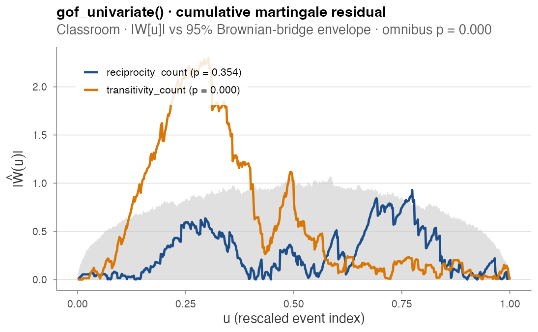

GOF cumulative process

reciprocity_count’s process (blue) stays inside the 95 % Brownian-bridge envelope; transitivity_count’s process (orange) shoots well above the envelope around u ≈ 0.30, where the running residual is most informative. The omnibus Cauchy combination rejects the overall model with p < 10⁻³ — and the per-component test pinpoints transitivity_count as the offender. The right next move is to enrich the transitivity term (try tv, nl, or a finer variant from the Endogenous catalogue) and re-test.

Function	Statistic	p-value
`gof_univariate`	`T_x = sup_u \|Ŵ[u]\|`	exact KS series (eq. 15)
`gof_multivariate`	`T_ψ = sup_u ‖Ŵ[u]‖²`	`n_sim` simulated q-dim Brownian bridges
`gof_global`	`T_o = mean tan(π(½ − P_l))`	`½ − arctan(T_o)/π` (Liu & Xie 2020)
`gof_auxiliary`	`T_φ = sup_u \|G[u]\|/√n`	`n_sim` standard-normal multipliers

These tests are complementary to the AIC-based selection performed by compare_models*(): AIC ranks competing fits, GOF tests check that the ranked-best fit is actually adequate.

These p-values are well calibrated under the null and for bounded statistics, but become anti-conservative for unbounded count statistics in the presence of a real effect — read them as diagnostic there. See the GoF calibration article for the empirical study and guidance.

Pointwise diagnostic · `martingale_residuals()`

For a more granular per-observation view, martingale_residuals() returns one row per case-control observation with the residual M_i = y_i − π_i where π_i = exp(η_i) / (exp(η_case) + exp(η_ctrl)) is the fitted probability that observation i is the case in its two-element risk set:

res <- martingale_residuals(
  classroom_events,
  model = c(reciprocity_count  = "linear",
            transitivity_count = "linear"),
  seed = 7)
# Residuals sum to zero within each (case, control) stratum:
#> Min       1st Qu    Median    Mean    3rd Qu    Max
#> -1.7e-16 -5.6e-17   0.0e+00  -3.6e-18 4.1e-17   2.2e-16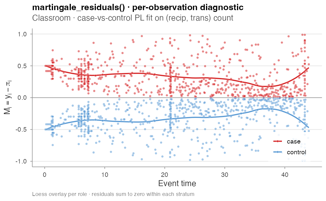

Martingale residuals over time

The within-stratum zero-sum invariant holds to machine precision. The loess overlays per role would land on zero under correct specification; the visible separation here is consistent with the GOF rejection above. Currently linear-effect specs only.

The neural backend

amorem ships a neural estimation backend, rem(method = "nn") (described above): a single multilayer perceptron scores every candidate in a case-control stratum, trained by Adam on the conditional-logistic partial likelihood. Because it scores the full covariate vector jointly, it can capture interactions between endogenous statistics that the additive gam backend cannot — at the cost of a coefficient table (effects are recovered post-hoc via partial-dependence plots) and, for now, of uncertainty quantification. The implementation is pure R with no extra dependencies, so it is reachable directly from install.packages(). See the Validation experiments for a gradient-correctness check and an interaction-recovery comparison against the linear backend.

The same training machinery also offers an additive-spline architecture — the STREAM construction of Filippi-Mazzola & Wit (2024, JRSS-C 73(4)): each covariate gets a B-spline expansion, a single linear layer over the concatenated bases yields sum_k f_k(x_k), and the model is trained by (mini-batch) stochastic gradient on the exact case-control partial likelihood. This keeps GAM-style interpretability (per-feature curves via plot(type = "pdp")) while batch_strata mini-batching scales to event logs far beyond what an in-memory smooth fit can hold:

fit_add <- rem(IS_OBSERVED ~ individual.activity + dyadic.activity,
               data = lesmis, method = "nn", stratum = "EVENT_INTERVAL",
               nn = nn_control(architecture = "additive_spline",
                               spline_df = 8, batch_strata = 512, seed = 1))
plot(fit_add$fit, type = "pdp")   # the fitted additive spline curves

Future directions. An optional torch engine for depth and GPU, factor embeddings (a neural analogue of re()), and uncertainty quantification for method = "nn" are natural extensions.

Estimation

Estimation

Case-control sampling

rem() · unified fitter for preprocessed data

compare_models() · linear AIC table

Actor random effects

compare_models_smooth() · TV / NL / TVNL effects

compare_models_global() · global covariate effects

Recency preprocessing

Goodness-of-fit · cumulative martingale residual tests

Pointwise diagnostic · martingale_residuals()

The neural backend

`rem()` · unified fitter for preprocessed data

`compare_models()` · linear AIC table

`compare_models_smooth()` · TV / NL / TVNL effects

`compare_models_global()` · global covariate effects

Pointwise diagnostic · `martingale_residuals()`