Real-data analysis

Three reproducible analyses on the bundled datasets. Every numerical and graphical output below is produced by paper/wiki/experiments/realdata.R.

Classroom · sender frailty flips the AIC ranking

The central methodological lesson of Juozaitienė & Wit (2024): without an actor-heterogeneity correction the *_count family silently absorbs sender activity differences, so it dominates the AIC table even when timing variants are the better description of the dynamics. Adding a Gamma survival::frailty() on the sender flips the ranking.

data(classroom_events)
specs <- list(
  count       = c("reciprocity_count", "transitivity_count"),
  continuous  = c("reciprocity_time_recent", "transitivity_time_recent"),
  interrupted = c("reciprocity_time_recent_interrupted",
                  "transitivity_time_recent_interrupted"))

compare_models(classroom_events, specs, n_controls = 3, seed = 11)
#>         model n_terms n_obs  log_lik      AIC delta_AIC
#> 1       count       2   691 -5248.2 11880.5     0.0
#> 2  continuous       2   691 -5368.1 12120.2   239.7
#> 3 interrupted       2   691 -5449.8 12283.6   403.1

compare_models(classroom_events, specs, n_controls = 3, seed = 11,
               random_effects = "sender")
#>         model n_terms n_obs  log_lik      AIC delta_AIC
#> 1  continuous       2   691 -5177.7 11776.8     0.0
#> 2 interrupted       2   691 -5269.4 11960.5   183.7
#> 3       count       2   691      NA      NA     NA       # convergence failure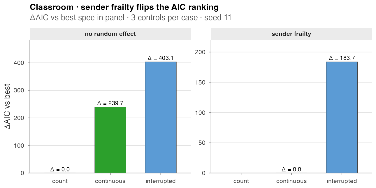

Classroom flip

Two findings worth flagging:

Count “wins” naively by 240 AIC over continuous (left panel). This is the trap the count family puts you in on datasets with heterogeneous senders.
With sender frailty (right panel) the count specification no longer fits — coxph(... + frailty(sender, ...)) fails its inner Newton–Raphson update once the random effect absorbs the activity differences. Continuous overtakes interrupted by 184 AIC points, matching Table 3 of Juozaitienė & Wit (2024).

Total wall-clock for the two compare_models calls: ~3 minutes. Driver: paper/wiki/experiments/realdata.R, section (a).

Manufacturing · smooth effect curves

A stratified Cox model with pspline(stat, df = 4) on four endogenous statistics (reciprocity_time_recent, transitivity_time_recent, and the interrupted variants of each), fit on the first 30 days of the radoslaw_email dataset (10,776 events, 151 actors) with three controls per case:

data(radoslaw_email)
re30 <- radoslaw_email[radoslaw_email$time < 30, ]
re30 <- re30[re30$sender != re30$receiver, ]

stat_names <- c("reciprocity_time_recent",
                "transitivity_time_recent",
                "reciprocity_time_recent_interrupted",
                "transitivity_time_recent_interrupted")

cc   <- sample_non_events(re30, n_controls = 3, seed = 11)
feat <- endogenous_features(cc, stats = stat_names)

fit <- survival::coxph(
  survival::Surv(rep(1, nrow(feat)), event) ~
    pspline(reciprocity_time_recent,            df = 4) +
    pspline(transitivity_time_recent,           df = 4) +
    pspline(reciprocity_time_recent_interrupted, df = 4) +
    pspline(transitivity_time_recent_interrupted, df = 4) +
    survival::strata(stratum),
  data = feat, method = "breslow")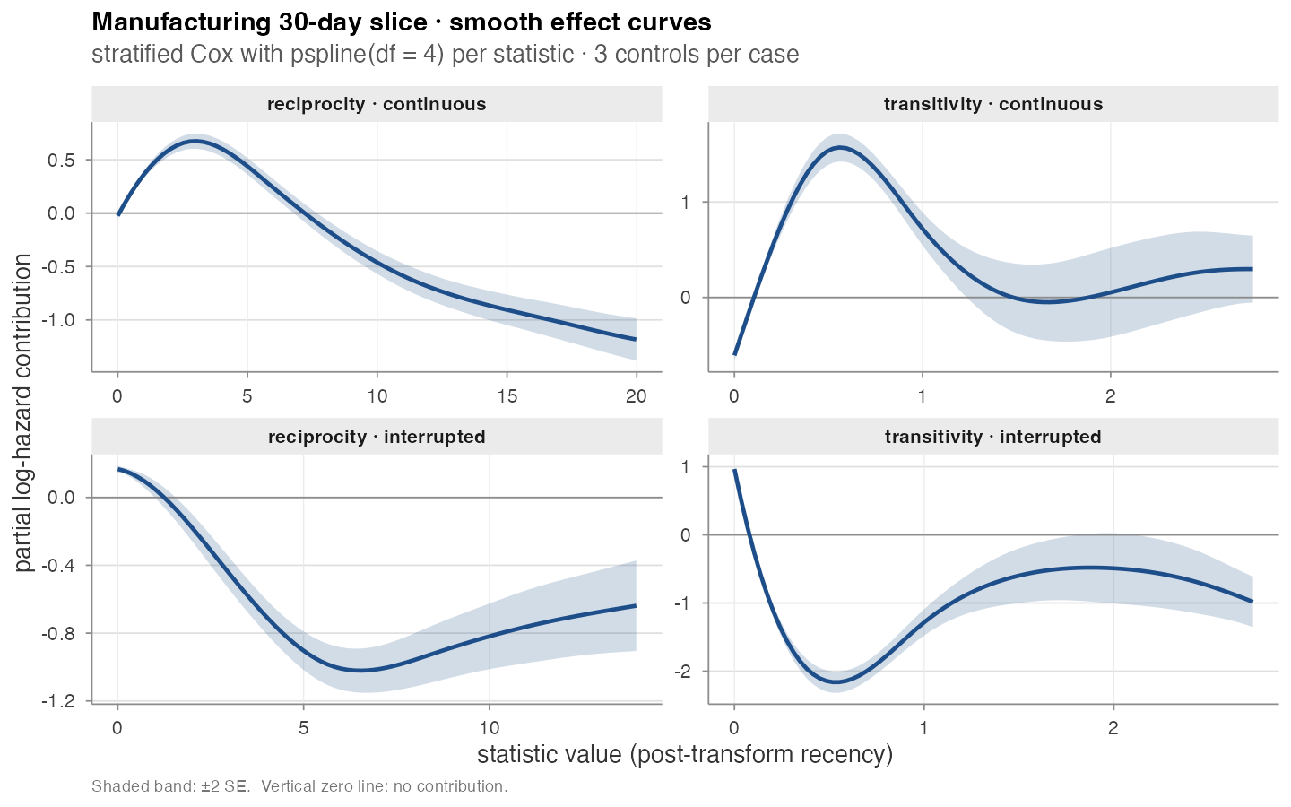

Smooth effect curves

The four panels are not redundant:

Continuous variants (top row) show the canonical “boost-then-decay” shape — a recent event raises the hazard briefly, then the contribution falls off and turns negative.
Interrupted variants (bottom row) start near zero, dip to a pronounced minimum, and partially recover. This is the cycle-closure-reset behavior the interrupted family is built to expose: once the closing event fires the statistic snaps to a fresh state, and the partial effect on subsequent events reflects that reset.

Fit wall-clock: ~40 s. Driver: section (b) of the same script.

CollegeMsg · first 30 days

A sanity check on the newly bundled college_msg dataset (60k IMs, 1899 users, 193 days; see Datasets). The first 30 days alone hold 22,265 messages across 1,086 users:

data(college_msg)
cm30 <- college_msg[college_msg$time < 30, ]
compare_models(cm30, specs, n_controls = 1, seed = 11)
#>         model n_terms  n_obs  log_lik      AIC  delta_AIC
#> 1       count       2  22265   -6775   13554        0
#> 2  continuous       2  22265  -14982   29968    16414
#> 3 interrupted       2  22265  -15059   30122    16567

The same pattern as Classroom — *_count “wins” by tens of thousands of AIC points because CollegeMsg has dramatic activity heterogeneity (see the actor-degree panel on the Datasets page). This is the kind of dataset where the sender-frailty correction is not optional; the naive ranking is not a reflection of the dynamics, it is a reflection of who happens to be highly active in the data.

Driver: section (c) of the same script. Runtime: ~30 s.