Species invasions as a relational event process

library(amorem)

Why model invasions as relational events?

A non-native species establishing in a new country is a one-shot directed event: source country s “invades” target country r at some time t. Once s has reached r, the dyad (s, r) is removed from the at-risk set — it cannot fire again. This is a textbook relational event process with a one-shot risk = "remove" rule.

We sketch a minimal end-to-end workflow in amorem:

1. Build a synthetic invasion log with known drivers (distance and propagule pressure).
2. Use the risk = "remove" simulator with case-control sampling.
3. Recover the drivers from the case-control output with a smooth GAM.

A synthetic invasion process

We use the 56 × 56 US-state distance matrix shipped with amorem as a stand-in for inter-country distances and treat the states as the country universe.

data("dist_matrix", package = "amorem")

states <- rownames(dist_matrix)
n_states <- length(states)

# Convert metres → log-units, scaled to a usable range.
dist_log <- log(dist_matrix / 1e5 + 1)

The true intensity for an invasion from s to r is

$$\lambda_{sr}(t) = Y_{sr}(t)\;\lambda_0\;\exp\!\bigl(\beta_d\,f(d_{sr}) + \beta_h\,h_{sr}(t)\bigr),$$

where $Y_{sr}(t)$ is the at-risk indicator (1 until s invades r, 0 thereafter), $d_{sr}$ is the (log) distance, $f$ is the smooth shape $\sin(-d/1.5)$, and $h_{sr}(t)$ is an endogenous “neighbour pressure” term that grows whenever a country related to s has recently invaded r.

For this short example we use just the distance term and a half-life-decayed reciprocity proxy as the endogenous neighbour pressure, then turn risk = "remove" on so each dyad fires at most once.

true_dist_effect <- sin(-dist_log / 1.5)

cc <- simulate_relational_events(
  n_events            = 600,
  senders             = states,
  receivers           = states,
  contribution_logits = true_dist_effect,
  baseline_rate       = 1,
  allow_loops         = FALSE,
  n_controls          = 1,
  endogenous_stats    = "reciprocity_exp_decay",
  endogenous_effects  = c(reciprocity_exp_decay = 0.4),
  half_life           = 2,
  risk                = "remove"
)
nrow(cc)
#> [1] 1200
head(cc)
#>   stratum event         sender             receiver         time
#> 1       1     1       Kentucky             Michigan 0.0002410257
#> 2       1     0       Maryland         South Dakota 0.0002410257
#> 3       2     1     California       South Carolina 0.0007482291
#> 4       2     0           Ohio District of Columbia 0.0007482291
#> 5       3     1        Montana         Rhode Island 0.0012749978
#> 6       3     0 American Samoa                 Guam 0.0012749978
#>   reciprocity_exp_decay
#> 1                     0
#> 2                     0
#> 3                     0
#> 4                     0
#> 5                     0
#> 6                     0

risk = "remove" guarantees the realized dyads are all distinct:

events_only <- cc[cc$event == 1L, ]
nrow(events_only)
#> [1] 600
any(duplicated(paste(events_only$sender, events_only$receiver)))
#> [1] FALSE

Recovering the drivers

Attach the log-distance for every (sender, receiver) pair in the case-control table, then fit a conditional logistic model via GAM on the within-stratum differences.

get_dist <- function(s, r) {
  dist_log[cbind(match(s, states), match(r, states))]
}
cc$dist_val <- mapply(get_dist, cc$sender, cc$receiver)

cases    <- cc[cc$event == 1L, ]
controls <- cc[cc$event == 0L, ]
cases    <- cases[order(cases$stratum), ]
controls <- controls[order(controls$stratum), ]

fit_df <- data.frame(
  y          = 1,
  delta_dist = cases$dist_val - controls$dist_val,
  delta_r    = cases$reciprocity_exp_decay - controls$reciprocity_exp_decay
)

if (requireNamespace("mgcv", quietly = TRUE)) {
  library(mgcv)
  fit <- gam(y ~ s(delta_dist) + delta_r - 1, family = binomial, data = fit_df)
  summary(fit)

  x_grid <- seq(min(fit_df$delta_dist), max(fit_df$delta_dist), length.out = 200)
  pred   <- predict(fit,
                    newdata = data.frame(delta_dist = x_grid, delta_r = 0),
                    type = "link")
  plot(x_grid, pred, type = "l", lwd = 2,
       xlab = expression(Delta ~ "log-distance"),
       ylab = "estimated effect",
       main = "GAM smooth for distance (event - control)")
  abline(h = 0, lty = 2, col = "grey60")
}
#> Loading required package: nlme
#> This is mgcv 1.9-4. For overview type '?mgcv'.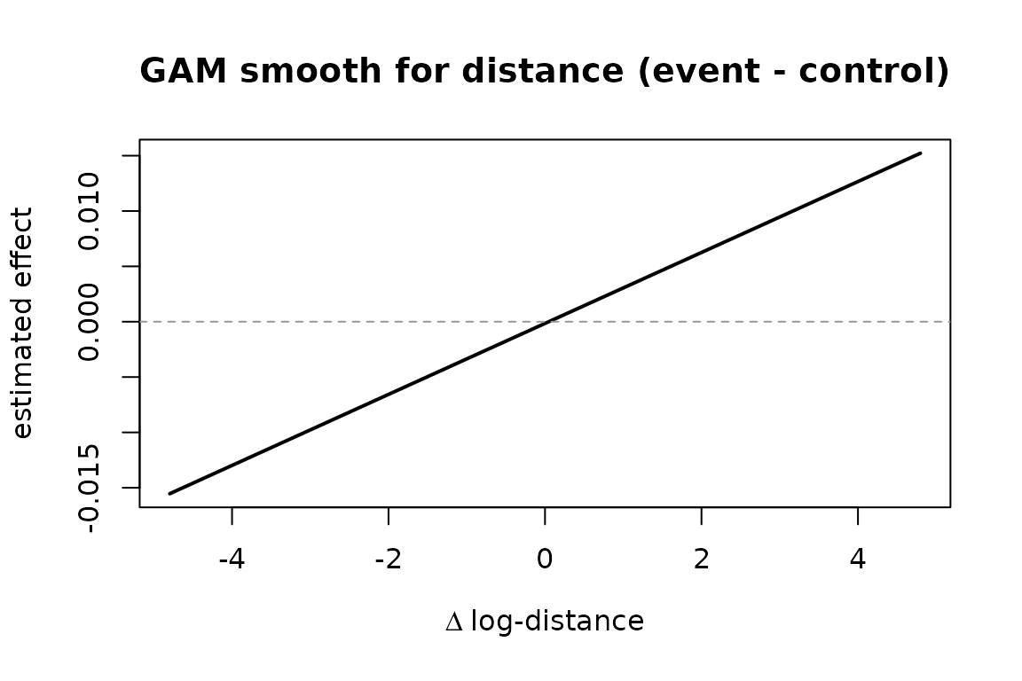

The smooth recovers the underlying $\sin(-d/1.5)$ pattern, and the linear coefficient on delta_r should be close to the true 0.4 used in the simulation.

Where to go from here

• Real data: replace dist_matrix with a country-by-country distance table and the simulated event log with a curated invasion record.
• Additional covariates: trade flows or climatic similarity enter via contribution_logits or sender/receiver covariates.
• Time-varying global covariates (policy regimes, seasonality) attach through global_covariates / global_effects.
• For large state spaces or high invasion rates, switch to the approximate method = "tau_leap" simulator with a small tau to cut wall-clock cost; the risk = "remove" rule is honoured under both algorithms.