Case study: international football, 1872

International football as an undirected event process

football_results lists every men’s international match since the first one, Scotland against England on 30 November 1872. A match is an undirected relational event: two national teams meet at a time. This case study asks what makes a pairing happen. Do the same teams meet again soon after a meeting (rivalries)? Do teams that share opponents meet each other (triadic closure)? Does a regional structure, visible in the network, raise the rate of pairs within a region? And do friendlies follow the same rules as competitive matches?

data(football_results)
f <- football_results
f$a <- pmin(f$sender, f$receiver)     # one order per pair: the match is undirected
f$b <- pmax(f$sender, f$receiver)
f$t <- as.numeric(f$date) / 365.25 + 1970   # decimal years
c(matches = nrow(f), teams = length(unique(c(f$a, f$b))),
  first = format(min(f$date)), last = format(max(f$date)))
#>      matches        teams        first         last 
#>      "49945"        "337" "1872-11-30" "2026-10-06"

36.6% of the matches are friendlies. In the 36,669 matches played at one team’s home ground, the home team wins 50.7% and loses 26.4%; at neutral venues the first-listed team wins 44.2%. The data have no confederation column; the regional structure below is found from the matches themselves.

Who plays whom

The network of the 1990–2019 matches among the 120 most active teams. Each team is joined to the three opponents it met most often; groups are found by modularity (Louvain) on all their matches.

par(mar = c(0.5, 0.5, 2.6, 0.5))
nodes <- data.frame(id = lay$id, x = lay$x, y = lay$y, size = as.numeric(act[lay$id]),
                    col = gcol[as.character(lay$group)], label = lay$id)
e <- pt[keep, ]
same <- lay$group[match(e$from, lay$id)] == lay$group[match(e$to, lay$id)]
draw_network(nodes, data.frame(from = e$from, to = e$to, w = e$w,
                               col = ifelse(same, gcol[as.character(lay$group[match(e$from, lay$id)])], "#B4BBC0")),
             label_cex = 0.42, node_scale = c(0.5, 2.2))
for (g in names(gsize)) {   # name each group beside its cluster
  k <- lay$group == as.character(g)
  text(mean(lay$x[k]), max(lay$y[k]) + 0.045, paste(gname[[g]], "group"), col = gcol[[g]], font = 2, cex = 0.72, xpd = TRUE)
}
title_left("National teams play within their region",
           sprintf("1990-2019; each team joined to its 3 most frequent opponents (width: matches); dot size: matches played; colours: groups found by modularity; %s of matches within a group",
                   pct(n_within / sum(pt$w), 0)))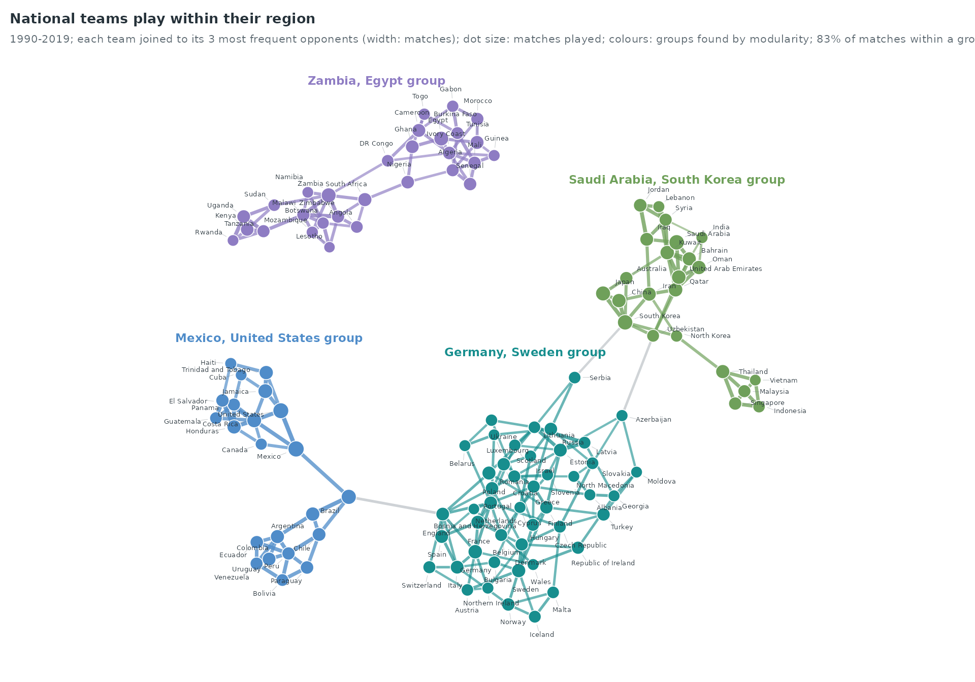

Network of national teams 1990-2019, coloured by regional group

The 4 groups follow geography: Germany, Sweden (46 teams); Zambia, Egypt (29 teams); Saudi Arabia, South Korea (23 teams); Mexico, United States (22 teams). 82.7% of the matches between these 120 teams are played within a group.

G <- grp_all[match(pt$from, top)]; H <- grp_all[match(pt$to, top)]
M <- tapply(pt$w, list(factor(G, names(gsize)), factor(H, names(gsize))), sum)
M[is.na(M)] <- 0
M <- (M + t(M)) / 2                       # undirected: half each way
dimnames(M) <- list(gname, gname)
par(mar = c(0.5, 3, 2.6, 3))
chord(M, setNames(gcol, gname), label_cex = 0.58)
title_left("Most matches stay inside a group", "1990-2019, 120 most active teams; ribbon width: number of matches")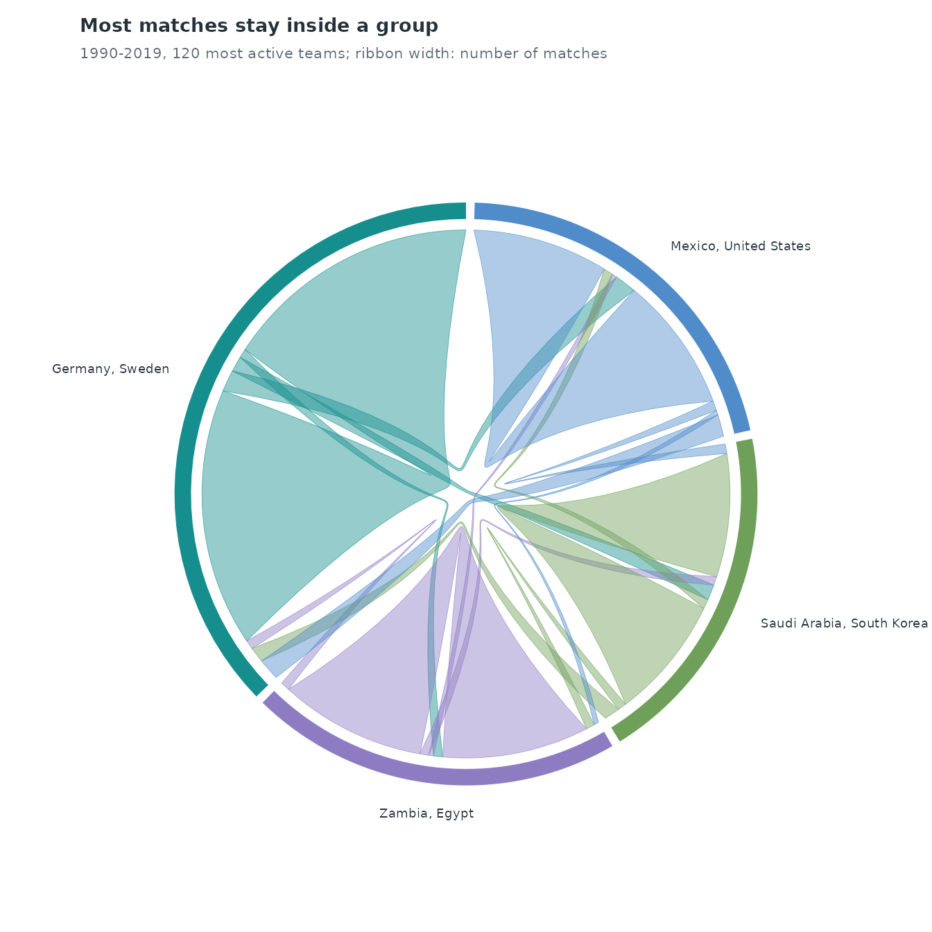

Chord diagram of matches between regional groups

Rivalries: the same pairs, again and again

The counting processes of the eight pairs that have met most often since 1872:

pc <- sort(table(paste(f$a, f$b, sep = " – ")), decreasing = TRUE)[1:8]
grid <- seq(1872, max(f$t), by = 0.25)
N <- sapply(names(pc), function(p) findInterval(grid, sort(f$t[paste(f$a, f$b, sep = " – ") == p])))
par(mar = c(3, 3.6, 2.6, 11))
matplot(grid, N, type = "s", lty = 1, lwd = 2, col = pal[1:8], axes = FALSE, xlab = "", ylab = "", xaxs = "i")
axis(1, tick = FALSE, cex.axis = 0.75, col.axis = ink_soft, line = -0.5)
axis(2, las = 1, tick = FALSE, cex.axis = 0.75, col.axis = ink_soft, line = -0.5)
end <- N[nrow(N), ]; o <- order(end); ya <- end; yy <- end[o]
for (i in seq_along(yy)[-1]) yy[i] <- max(yy[i], yy[i - 1] + diff(par("usr")[3:4]) * 0.055)
ya[o] <- yy
text(par("usr")[2], ya, paste0(names(pc), "  ", pc), pos = 4, xpd = TRUE, cex = 0.62, col = pal[1:8])
title_left("Rivalries accumulate over a century", "cumulative matches N(t) of the eight most frequent pairings")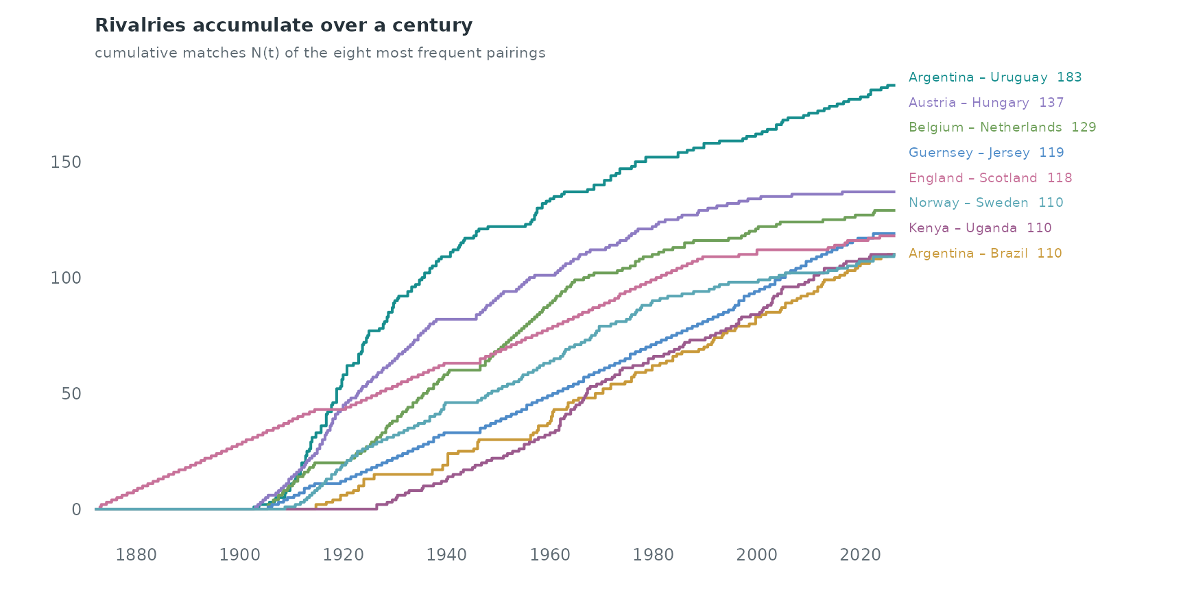

Cumulative number of matches of the eight most frequent pairings since 1872

Argentina – Uruguay have met 183 times. The flat stretches of 1914–1918 and 1939–1945 are the two world wars.

The whole record, four years at a time, on a fixed layout of the 80 teams with most matches since 1872 (colours: the groups of the network above; grey: teams outside it):

From 4 matches in 1872–1875, the record grows to 4,008 in 2008–2011. The regional groups fill in one after another: the median team of each group played its first international in 1922 (Germany, Sweden group), 1922 (Mexico, United States group), 1953 (Saudi Arabia, South Korea group), 1958 (Zambia, Egypt group).

A relational event model for pairings

We model the matches of 1990–2019 (26,282 matches). For each match, sample_non_events() draws one pair of teams that had both played before (scope = "appearance"); it is run on the whole record since 1872 so that “played before” counts every earlier match, and only the 1990–2019 strata are kept. The sampler draws ordered pairs; each control is put in the same alphabetical order as the matches.

hist <- f[f$t < 2020, c("a", "b", "t", "tournament")]
hist <- hist[order(hist$t), ]
cc <- sample_non_events(data.frame(sender = hist$a, receiver = hist$b, time = hist$t),
                        scope = "appearance", seed = 1)
cc <- cc[cc$time >= 1990, ]
swap <- cc$sender > cc$receiver
cc[swap, c("sender", "receiver")] <- cc[swap, c("receiver", "sender")]
table(cc$event)
#> 
#>     0     1 
#> 26282 26282

endogenous_features() computes directed statistics, so the undirected ones are computed here from the match history strictly before each row’s time, over the previous ten years:

activity: matches played by each of the two teams;
common opponents: teams that both have played (triadic closure);
repetition: earlier matches between the two teams;
years since the last meeting, at any time since 1872, with an indicator for pairs that have never met.

und_stats <- function(i, j, t, hist, window = 10) {
  team <- c(hist$a, hist$b); opp <- c(hist$b, hist$a); tt <- c(hist$t, hist$t)
  o <- order(team, tt); team <- team[o]; opp <- opp[o]; tt <- tt[o]
  first <- match(unique(team), team); names(first) <- unique(team)
  last <- c(first[-1] - 1, length(team)); names(last) <- names(first)
  pt <- split(hist$t, paste(hist$a, hist$b, sep = "|"))
  recent <- function(x, s) {       # matches of team x in [s - window, s)
    if (is.na(first[x])) return(list(n = 0, opp = character(0)))
    r <- first[x]:last[x]; tx <- tt[r]
    hi <- findInterval(s, tx, left.open = TRUE); lo <- findInterval(s - window, tx, left.open = TRUE)
    k <- if (hi > lo) r[(lo + 1):hi] else integer(0)
    list(n = length(k), opp = unique(opp[k]))
  }
  out <- t(vapply(seq_along(i), function(k) {
    a <- recent(i[k], t[k]); b <- recent(j[k], t[k])
    p <- pt[[paste(i[k], j[k], sep = "|")]]; p <- p[p < t[k]]
    c(act_i = a$n, act_j = b$n, common = length(intersect(a$opp, b$opp)),
      pair = sum(p >= t[k] - window), since = if (length(p)) t[k] - max(p) else NA)
  }, numeric(5)))
  as.data.frame(out)
}
cc <- cbind(cc, und_stats(cc$sender, cc$receiver, cc$time, hist))

The regional groups for the model are found on the 1960–1989 matches, so that the grouping does not use the matches it is meant to explain. Teams that did not play then (many post-1990 states among them) belong to no group.

old <- f[f$t >= 1960 & f$t < 1990, ]
old_pairs <- aggregate(list(w = rep(1, nrow(old))), list(from = old$a, to = old$b), sum)
g_old <- layout_graph(old_pairs)
grp <- setNames(g_old$group, g_old$id)
cc$same_group <- as.integer(!is.na(grp[cc$sender]) & !is.na(grp[cc$receiver]) &
                            grp[cc$sender] == grp[cc$receiver])
cc$never <- as.integer(is.na(cc$since))
cc$log_since <- log(ifelse(is.na(cc$since), max(cc$since, na.rm = TRUE), cc$since))
cc$log_activity <- log1p(cc$act_i) + log1p(cc$act_j)
cc$log_common <- log1p(cc$common)
cc$log_pair <- log1p(cc$pair)
aggregate(cbind(act_i, common, pair, never) ~ event, cc, mean)
#>   event    act_i    common      pair     never
#> 1     0 58.30538  3.075527 0.2207975 0.8722319
#> 2     1 88.36725 17.334411 2.7739518 0.1584735

cv <- c("log_activity", "log_common", "log_pair", "same_group", "never", "log_since")
w <- widen_case_control(cc, covariates = cv)
fit <- rem(~ log_activity + log_common + log_pair + same_group + never + nl(log_since, k = 6),
           data = w, method = "gam")
est <- summary(fit)$p.table[, c("Estimate", "Std. Error")]
round(est, 3)
#>              Estimate Std. Error
#> log_activity   -0.357      0.018
#> log_common      1.801      0.040
#> log_pair        0.189      0.068
#> same_group      0.446      0.051
#> never          -0.281      0.287

d <- smooth_data(fit$fit, 1)                      # x is log(years)
lo <- d$fit - 1.96 * d$se; hi <- d$fit + 1.96 * d$se
par(mar = c(3.4, 3.8, 2.6, 1))
plot(d$x, d$fit, type = "n", ylim = range(lo, hi, 0), axes = FALSE, xlab = "", ylab = "")
abline(h = 0, col = rule, lwd = 1.2)
polygon(c(d$x, rev(d$x)), c(lo, rev(hi)), col = alpha(pal[1], 0.18), border = NA)
lines(d$x, d$fit, col = pal[1], lwd = 2.2)
yrs <- c(1 / 52, 1 / 12, 0.5, 1, 2, 5, 10, 20, 50, 100)
yrs <- yrs[log(yrs) >= min(d$x) & log(yrs) <= max(d$x)]
axis(1, at = log(yrs), labels = c("1 week", "1 month", "6 months", "1", "2", "5", "10", "20", "50", "100")[
  match(yrs, c(1 / 52, 1 / 12, 0.5, 1, 2, 5, 10, 20, 50, 100))], tick = FALSE, cex.axis = 0.75, col.axis = ink_soft, line = -0.5)
axis(2, las = 1, tick = FALSE, cex.axis = 0.75, col.axis = ink_soft, line = -0.5)
mtext("years since the two teams last met (log scale)", side = 1, line = 2, cex = 0.75, col = ink_soft)
mtext("effect on the log-rate", side = 2, line = 2.3, cex = 0.75, col = ink_soft)
y1 <- d$fit[which.min(abs(d$x - log(1)))]; y10 <- d$fit[which.min(abs(d$x - log(10)))]
points(log(c(1, 10)), c(y1, y10), pch = 21, bg = "white", col = ink, cex = 1.2, lwd = 1.4)
segments(log(1), y1, log(10), y1, col = ink_soft, lty = 3); segments(log(10), y1, log(10), y10, col = ink_soft, lty = 3)
text(mean(log(c(1, 10))), y1 + 0.45, sprintf("1 year vs 10 years: %s times the rate", fmt(exp(y1 - y10), 1)), cex = 0.7, col = ink)
title_left("A pairing is most likely soon after the last meeting",
           "smooth effect of the time since the last meeting, with 95% band; other terms held fixed")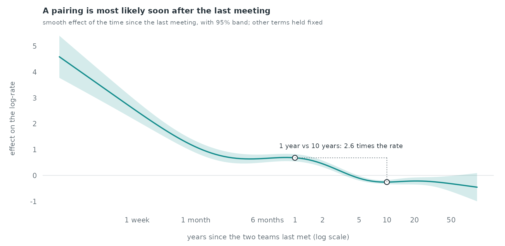

Smooth effect of years since the last meeting on the rate of a pairing, log axis

Pairs that meet again within days, the two legs of a tie or two matches of one tournament, have the highest rate. Holding the other terms fixed, a pairing whose last meeting was one year ago has a log-rate 0.94 higher than one that last met ten years ago (a factor of 2.6). Common opponents carry the largest linear effect, 1.80 per unit of log(1 + common opponents) (s.e. 0.04); a pair in the same 1960–1989 group has a log-rate 0.45 higher (s.e. 0.05). Activity enters with -0.36: given the common opponents, which grow with activity, more active teams do not meet each other more.

Friendlies and competitive matches

Each stratum holds one match and its control, so the strata of friendlies and of competitive matches give two separate partial likelihoods: the rate of a friendly and the rate of a competitive match between a pair. Both use the same statistics, with the time since the last meeting entering linearly.

type <- hist$tournament[match(paste(cc$sender, cc$receiver, cc$time)[cc$event == 1],
                              paste(hist$a, hist$b, hist$t))]
cc$friendly <- (type == "Friendly")[match(cc$stratum, cc$stratum[cc$event == 1])]
fits <- lapply(c(friendly = TRUE, competitive = FALSE), function(fr) {
  wd <- widen_case_control(cc[cc$friendly == fr, ], covariates = cv)
  summary(rem(~ log_activity + log_common + log_pair + same_group + never + log_since,
              data = wd, method = "gam"))$p.table[, 1:2]
})
sapply(fits, function(p) round(p[, 1], 3))
#>              friendly competitive
#> log_activity   -0.151      -0.487
#> log_common      1.610       1.924
#> log_pair        0.257       0.060
#> same_group      0.179       0.616
#> never          -0.051       0.277
#> log_since      -0.205      -0.416

lab <- c(log_activity = "activity of the two teams", log_common = "common opponents",
         log_pair = "earlier meetings (10 years)", same_group = "same regional group",
         never = "never met before", log_since = "log years since last meeting")
k <- length(lab); y <- k:1
par(mar = c(3.4, 13, 2.6, 1))
rng <- range(sapply(fits, function(p) c(p[, 1] - 1.96 * p[, 2], p[, 1] + 1.96 * p[, 2])), 0)
plot(NA, xlim = rng, ylim = c(0.5, k + 0.5), axes = FALSE, xlab = "", ylab = "")
abline(v = 0, col = rule, lwd = 1.2)
for (m in 1:2) {
  p <- fits[[m]][names(lab), ]; yy <- y + c(0.13, -0.13)[m]
  segments(p[, 1] - 1.96 * p[, 2], yy, p[, 1] + 1.96 * p[, 2], yy, col = pal[c(6, 4)][m], lwd = 2.2)
  points(p[, 1], yy, pch = 21, bg = "white", col = pal[c(6, 4)][m], cex = 1.2, lwd = 1.6)
}
axis(1, tick = FALSE, cex.axis = 0.75, col.axis = ink_soft, line = -0.5)
axis(2, at = y, labels = lab, las = 1, tick = FALSE, cex.axis = 0.75, col.axis = ink, line = -0.6)
mtext("effect on the log-rate, with 95% interval", side = 1, line = 2, cex = 0.75, col = ink_soft)
sgp <- sapply(fits, function(p) p["same_group", 1])
text(max(sgp) + 0.12, y[names(lab) == "same_group"], sprintf("%s vs %s", fmt(sgp[["friendly"]], 2), fmt(sgp[["competitive"]], 2)),
     adj = 0, cex = 0.7, col = ink, font = 2)
legend("bottomright", c("friendlies", "competitive matches"), col = pal[c(6, 4)], pch = 21, pt.bg = "white",
       lwd = 2, bty = "n", cex = 0.72, text.col = ink)
title_left("Region matters more for competitive matches", "1990-2019, one model per match type")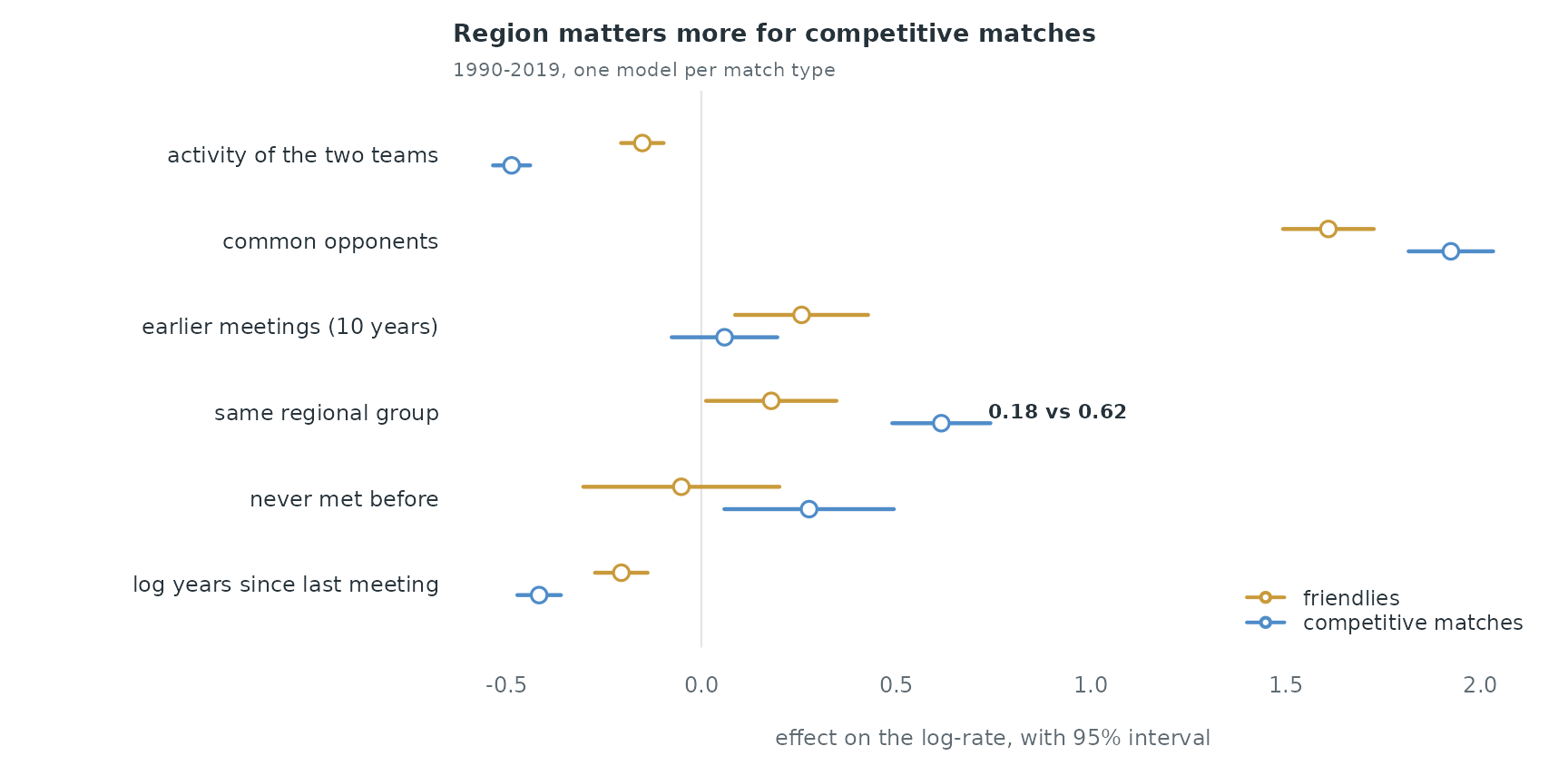

Coefficients for friendlies and competitive matches side by side

The same-group coefficient is 0.62 for competitive matches and 0.18 for friendlies: qualifying competitions are organised by confederation, while friendlies are arranged across regions. The rate of a competitive match also falls faster with the time since the last meeting (-0.42 against -0.21 per unit of log years), as qualifying groups bring the same teams together in successive cycles.

What is not in the model