Analyses of bundled event logs

Three analyses on the bundled datasets. The code below runs when this page is built, so every table, figure and number in the text comes from the current version of the package.

Classroom · timing variants with and without a sender frailty

Juozaitienė & Wit (2024) compare count statistics with timing variants (time since the most recent reciprocating or transitive event, continuous or interrupted by a closing event). Count statistics also carry sender activity: an actor who sends a lot accumulates large counts. A Gamma sender frailty (random_effects = "sender") absorbs activity differences between senders.

data(classroom_events)
specs <- list(
  count       = c("reciprocity_count", "transitivity_count"),
  continuous  = c("reciprocity_time_recent", "transitivity_time_recent"),
  interrupted = c("reciprocity_time_recent_interrupted",
                  "transitivity_time_recent_interrupted"))

no_re <- compare_models(classroom_events, specs, n_controls = 3, seed = 11)
no_re
#>         model n_terms n_obs   log_lik      AIC delta_AIC
#> 1       count       2   691 -653.3589 1310.718    0.0000
#> 2 interrupted       2   691 -864.9598 1733.920  423.2017
#> 3  continuous       2   691 -919.1762 1842.352  531.6345

with_re <- compare_models(classroom_events, specs, n_controls = 3, seed = 11,
                          random_effects = "sender")
with_re
#>         model n_terms n_obs   log_lik      AIC delta_AIC
#> 1       count       2   691 -525.3774 1092.430    0.0000
#> 2 interrupted       2   691 -679.7356 1401.603  309.1735
#> 3  continuous       2   691 -769.7646 1581.834  489.4043

cols <- c(count = "#d62728", continuous = "#2ca02c", interrupted = "#1f77b4")
op <- par(mfrow = c(1, 2), mar = c(4, 4.5, 2.5, 1))
for (tab in list(no_re, with_re)) {
  d <- setNames(tab$delta_AIC, tab$model)[names(specs)]
  bp <- barplot(d, col = cols[names(d)], ylim = c(0, max(d) * 1.15),
                ylab = expression(Delta * "AIC"),
                main = if (identical(tab, no_re)) "no random effect" else "sender frailty")
  text(bp, d, sprintf("%.1f", d), pos = 3, cex = 0.85)
}

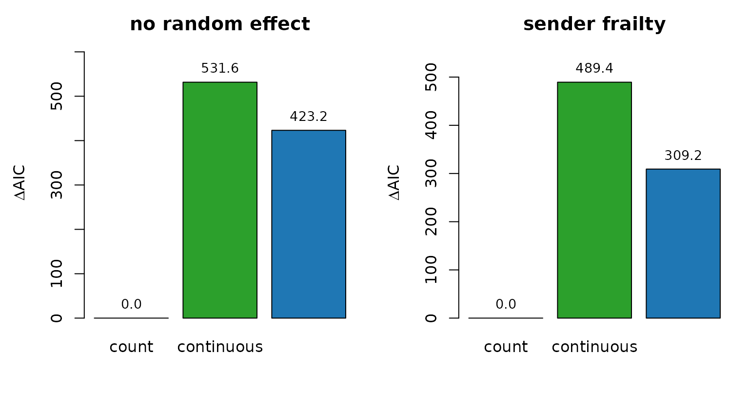
Delta AIC of the three specifications without and with a sender frailty

par(op)

Without a random effect the count specification has the lowest AIC, ahead of interrupted by 423.2. With the sender frailty the count specification still has the lowest AIC, and its lead over interrupted is 309.2. Among the timing variants, interrupted fits better than continuous by 180.2 AIC points once the frailty is in the model.

Manufacturing · smooth effect curves

A stratified Cox model with pspline(stat, df = 4) on four endogenous statistics, fitted on the first 30 days of the radoslaw_email dataset with three controls per case. Statistics are computed with the default endogenous_features() behaviour on case-control data: the controls are scored against the history of observed events without entering it. Each time gap is mapped to a recency weight with transform_recency() (1 for an event that just happened, falling towards 0 as the gap grows), and a dyad with no such event gets weight 0.

data(radoslaw_email)
re30 <- radoslaw_email[radoslaw_email$time < 30, ]
re30 <- re30[re30$sender != re30$receiver, ]

stat_names <- c("reciprocity_time_recent",
                "transitivity_time_recent",
                "reciprocity_time_recent_interrupted",
                "transitivity_time_recent_interrupted")

cc   <- sample_non_events(re30, n_controls = 3, seed = 11)
feat <- endogenous_features(cc, stats = stat_names)
for (s in stat_names) {
  w <- transform_recency(feat[[s]])
  w[is.na(w)] <- 0                     # no such event yet: weight 0
  feat[[s]] <- w
}

library(survival)   # coxph() recognises pspline() and strata() only unqualified
fit <- coxph(
  Surv(rep(1, nrow(feat)), event) ~
    pspline(reciprocity_time_recent,              df = 4) +
    pspline(transitivity_time_recent,             df = 4) +
    pspline(reciprocity_time_recent_interrupted,  df = 4) +
    pspline(transitivity_time_recent_interrupted, df = 4) +
    strata(stratum),
  data = feat, method = "breslow")
c(events = nrow(re30), actors = length(unique(c(re30$sender, re30$receiver))))
#> events actors 
#>  10776    151

panel <- c("reciprocity · continuous", "transitivity · continuous",
           "reciprocity · interrupted", "transitivity · interrupted")
op <- par(mfrow = c(2, 2), mar = c(4, 4.5, 2.5, 1))
for (j in seq_along(stat_names)) {
  s <- stat_names[j]
  rng <- stats::quantile(feat[[s]], c(0.02, 0.98))
  nd <- feat[rep(1, 80), ]
  for (o in stat_names) nd[[o]] <- stats::median(feat[[o]])
  nd[[s]] <- seq(rng[1], rng[2], length.out = 80)
  pr <- stats::predict(fit, newdata = nd, type = "terms", se.fit = TRUE)
  k <- grep(s, colnames(pr$fit), fixed = TRUE)[1]
  y <- pr$fit[, k]; se <- pr$se.fit[, k]
  plot(nd[[s]], y, type = "n", ylim = range(y - 2 * se, y + 2 * se),
       xlab = "recency weight", ylab = "partial log-hazard", main = panel[j])
  polygon(c(nd[[s]], rev(nd[[s]])), c(y + 2 * se, rev(y - 2 * se)),
          col = grDevices::adjustcolor("#1d4e89", 0.2), border = NA)
  abline(h = 0, col = "grey60")
  lines(nd[[s]], y, lwd = 2, col = "#1d4e89")
}

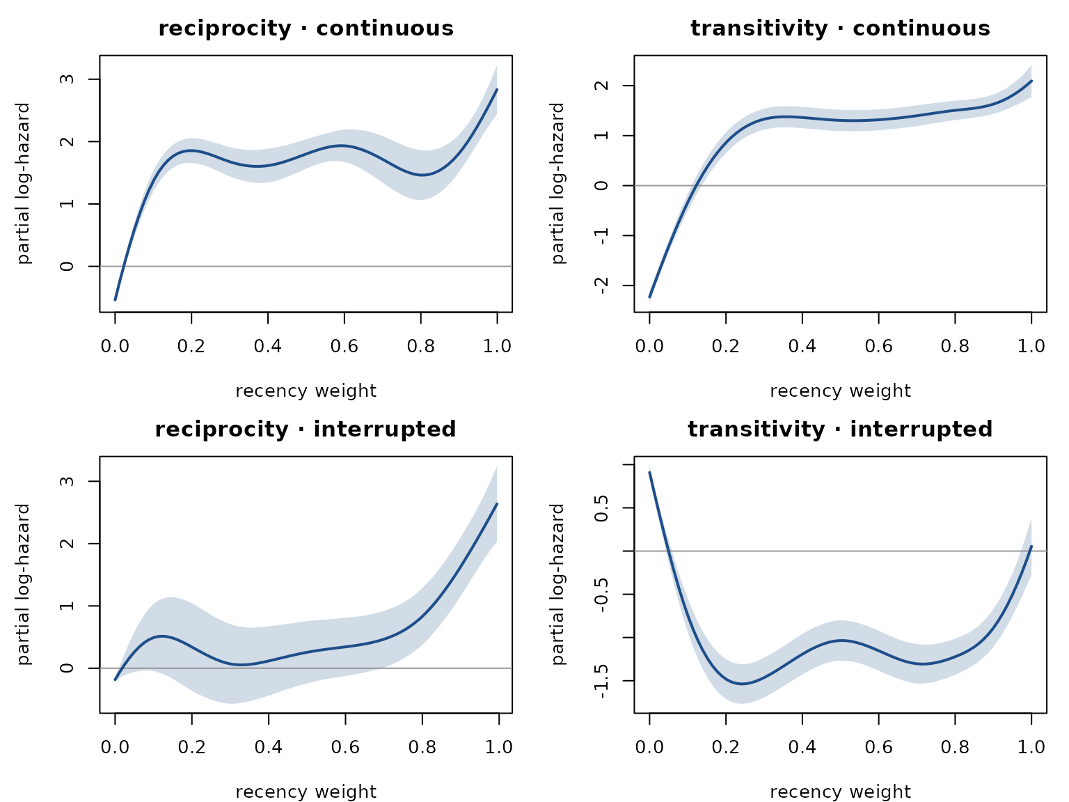
Smooth partial log-hazard contributions of the four timing statistics

par(op)

Each panel shows one statistic’s contribution to the log-hazard, with the other three held at their medians; the band is ±2 standard errors. In this fit the two continuous variants rise steeply from weight 0 (no reciprocating or transitive event yet) and stay high, peaking for the most recent events. The interrupted reciprocity curve stays near zero until large weights and then rises; the interrupted transitivity curve is highest at weight 0 and below zero for most of the range.

CollegeMsg · first 30 days

The same three specifications on the first 30 days of college_msg, with one control per case:

data(college_msg)
cm30 <- college_msg[college_msg$time < 30, ]
c(messages = nrow(cm30), users = length(unique(c(cm30$sender, cm30$receiver))))
#> messages    users 
#>    22265     1086
cm <- compare_models(cm30, specs, n_controls = 1, seed = 11)
cm
#>         model n_terms n_obs    log_lik      AIC delta_AIC
#> 1       count       2 22265  -6782.367 13568.73      0.00
#> 2  continuous       2 22265 -13853.169 27710.34  14141.60
#> 3 interrupted       2 22265 -14716.110 29436.22  15867.48

The count specification leads by 14,142 AIC points. The datasets article shows the activity heterogeneity of this network (see the actor-degree panel on the Datasets page); without a sender frailty the count statistics carry that heterogeneity, so this table ranks the specifications on activity as much as on dynamics.