Case study: time of day and day of week in company email

Time of day and day of week in company email

radoslaw_email records the internal email of a manufacturing company (Michalski et al. 2011; Nurek & Michalski 2020, a company in Poland). Email is sent during working hours and on working days, so the rate of every dyad depends on the clock. Time of day and day of week are global covariates: at any instant they take the same value for every sender–receiver pair. This case study estimates their effect next to an endogenous reciprocity effect, using time-shifted case-control sampling, and checks the fitted model with gof_rem(), gof_multivariate() and gof_auxiliary().

Data and clock time

time counts days since the first email; attr(radoslaw_email, "unix_origin") holds that instant as a Unix time. We use the first 30 days and convert each time to Central European clock time.

data(radoslaw_email)
origin <- attr(radoslaw_email, "unix_origin")
ev <- radoslaw_email[radoslaw_email$time < 30 &
                     radoslaw_email$sender != radoslaw_email$receiver,
                     c("sender", "receiver", "time")]

clock <- function(t) as.POSIXlt(origin + t * 86400, origin = "1970-01-01",
                                tz = "Europe/Warsaw")
tod <- function(t) { p <- clock(t); p$hour + p$min / 60 + p$sec / 3600 }  # hours
dow <- function(t) { p <- clock(t); (p$wday + 6) %% 7 + tod(t) / 24 }     # 0 = Monday 00:00

c(events = nrow(ev), actors = length(unique(c(ev$sender, ev$receiver))),
  first = format(clock(min(ev$time))), last = format(clock(max(ev$time))))
#>                events                actors                 first 
#>               "10776"                 "151" "2010-01-02 17:40:10" 
#>                  last 
#> "2010-02-01 17:35:37"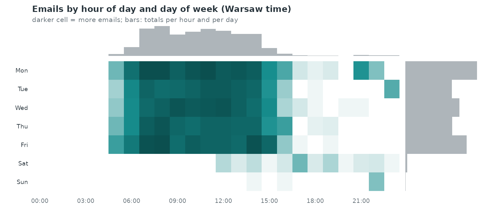

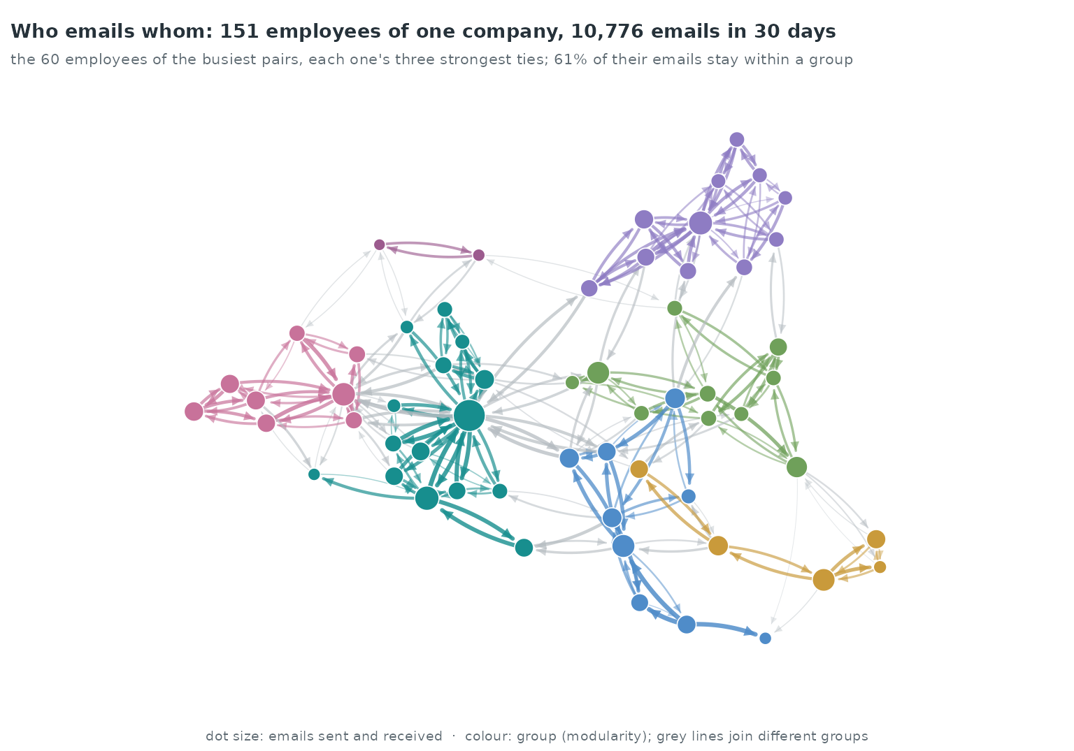
92.6% of the emails are sent between 07:00 and 16:00, and 0.8% on Saturday or Sunday.

The animation pools the 30 days by hour of the week, so each frame shows the emails sent in one 2-hour window of a Monday-to-Sunday week. The busiest window, Mon 10:00–12:00, carries 6.2% of the emails; 31 of the 84 windows have none.

Ordinary sampling cannot see a global covariate

With ordinary nested case-control sampling each control gets its event’s time, so a covariate that depends on time alone takes the same value for the event and its control:

cc0 <- sample_non_events(ev, seed = 1)
cc0$tod <- tod(cc0$time)
w0 <- widen_case_control(cc0, covariates = "tod")
summary(w0$d_tod)
#>    Min. 1st Qu.  Median    Mean 3rd Qu.    Max. 
#>       0       0       0       0       0       0

Every event-minus-control difference is zero, so the time-of-day effect drops out of the partial likelihood.

Time-shifted sampling

shift = "exponential" draws one exponential shift per dyad and samples each control from the dyads whose back-shifted time falls in the observation window (here the 30 days of the slice). Each control is stored at its own time.

cc <- sample_non_events(ev, seed = 1, shift = "exponential", window = c(0, 30))
sh <- attr(cc, "shift")
c(mean_shift_days = sh$mean, uninformative_events = length(sh$uninformative))
#>      mean_shift_days uninformative_events 
#>             15.23542              0.00000

The endogenous covariate is reciprocity timing: the time since the receiver last emailed the sender, mapped to a recency weight with transform_recency() (1 when the receiver emailed the sender a moment ago, falling towards 0 as the gap grows, and 0 when the receiver has not emailed the sender). On case-control data endogenous_features() builds the history from the observed emails only, and each control is scored at its own time. Time of day and day of week are read from each row’s clock time.

cc <- endogenous_features(cc, stats = "reciprocity_time_recent")
cc$recip <- transform_recency(cc$reciprocity_time_recent)
cc$recip[is.na(cc$recip)] <- 0
cc$tod <- tod(cc$time)
cc$dow <- dow(cc$time)
w <- widen_case_control(cc, covariates = c("recip", "tod", "dow", "time"))
summary(w$d_tod)
#>    Min. 1st Qu.  Median    Mean 3rd Qu.    Max. 
#> -18.314  -7.283  -1.169  -1.144   4.869  23.427

Model

Time of day and day of week enter as cyclic smooths (bs = "cc"), the residual trend over the 30 days as nl(time), and reciprocity as a time-varying effect tv(recip). Because the controls carry their own times, tv(recip) contributes $\beta(t)\,x_{ev} - \beta(t^*)\,x_{nv}$, with $t$ the event time and $t^*$ the control’s time.

fit <- rem(~ nl(tod, bs = "cc", k = 12) + nl(dow, bs = "cc", k = 8) +
             nl(time, k = 5) + tv(recip, k = 5),
           data = w, method = "gam", time = "time")
summary(fit)$s.table
#>                       edf    Ref.df    Chi.sq      p-value
#> s(.X_tod):.I     9.820934 10.000000 938.51277 0.0000000000
#> s(.X_dow):.I     5.931675  6.000000 433.23812 0.0000000000
#> s(.X_time):.I    3.167483  3.640323  22.21318 0.0003238577
#> s(.TP):.XI_recip 2.000223  2.000444 301.06346 0.0000000000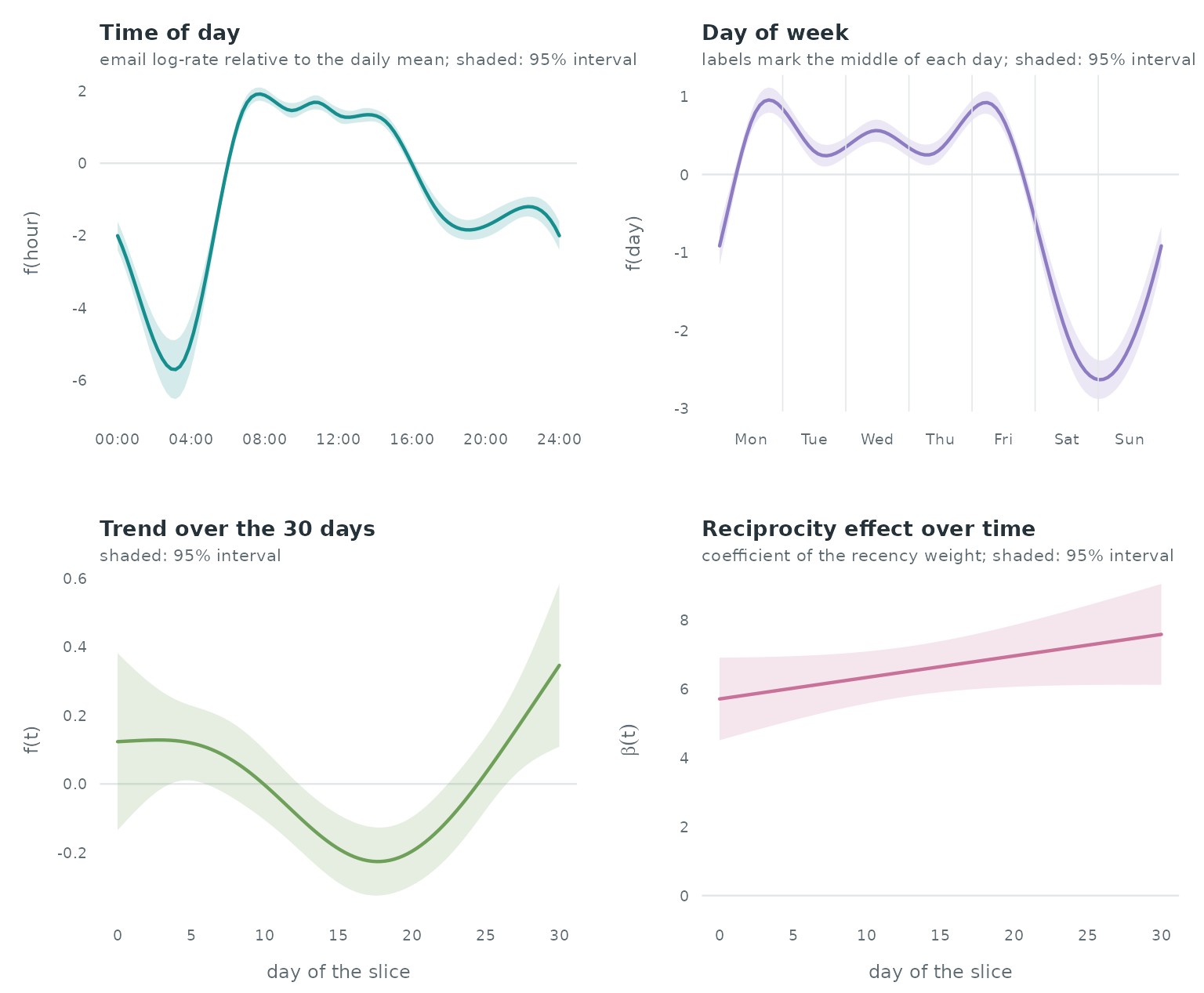

In the mgcv summary the largest p-value of the four smooth terms is 3.2e-04. The time-of-day curve is lowest at about 3.1 h and ranges from -0.04 to 1.88 between 08:00 and 16:00. The day-of-week curve averages 0.44 from Monday to Friday and -1.97 on Saturday and Sunday (log-rate scale, each curve centred by mgcv). Over the 30 days the reciprocity coefficient $\beta(t)$ ranges from 5.71 to 7.59. Shaded bands in the figure are 95% intervals.

Goodness of fit of the fitted model

gof_rem() tests the fitted model directly. The functional-form test orders the residuals by the covariate’s value, and the time test cumulates the residuals of a term over event time; both use a multiplier bootstrap that accounts for the estimated coefficients.

g_tod  <- gof_rem(fit, "tod", test = "functional_form", n_sim = 1000, seed = 1)
g_dow  <- gof_rem(fit, "dow", test = "functional_form", n_sim = 1000, seed = 1)
g_time <- gof_rem(fit, "recip", test = "time", data = w, n_sim = 1000, seed = 1)
g_tod; g_dow; g_time
#> Martingale-residual GoF test of 'tod': functional form
#>   sup statistic = 0.2554, p-value = 0.0000 (1000 bootstrap replicates, n = 10776)
#> Martingale-residual GoF test of 'dow': functional form
#>   sup statistic = 0.5011, p-value = 0.0000 (1000 bootstrap replicates, n = 10776)
#> Martingale-residual GoF test of 'recip': time specification
#>   sup statistic = 0.1370, p-value = 0.0020 (1000 bootstrap replicates, n = 10776)

op <- par(mfrow = c(1, 3), mar = c(4, 4, 2.5, 1))
plot(g_tod, main = "time of day: functional form")
plot(g_dow, main = "day of week: functional form")
plot(g_time, main = "reciprocity: time")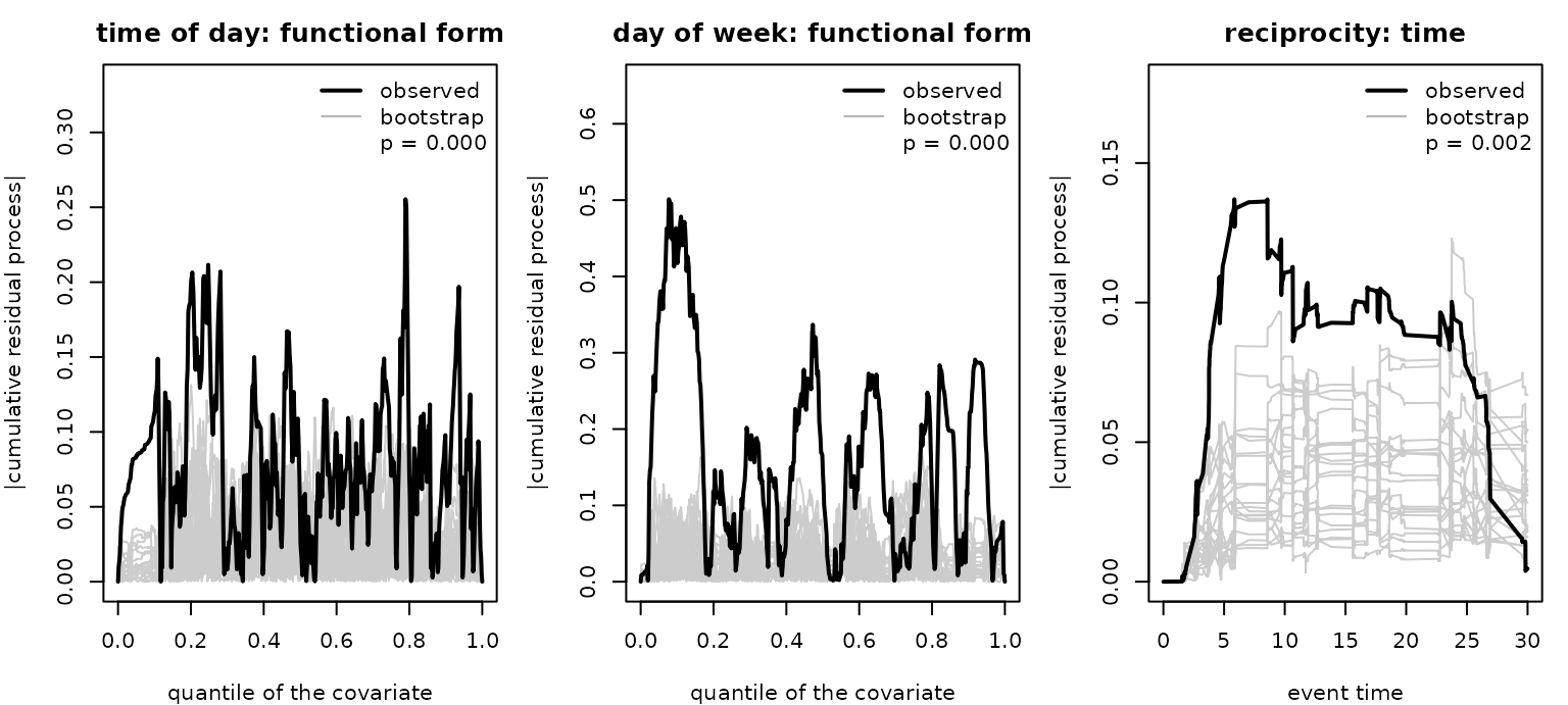

par(op)

The functional-form test gives p < 0.001 for time of day and p < 0.001 for day of week; the time test for the reciprocity term gives p = 0.002.

Linear-model diagnostics on one week

gof_multivariate() and gof_auxiliary() take an event log and a linear model, draw their own case-control sample and refit. Here they run on the first week of the slice with count statistics: gof_multivariate() tests whether reciprocity_count needs a smooth instead of a linear effect, and gof_auxiliary() tests whether an unmodelled statistic carries signal the model misses.

ev7 <- ev[ev$time < 7, ]
m <- c(reciprocity_count = "linear", transitivity_count = "linear")
gm <- gof_multivariate(ev7, m, covariate = "reciprocity_count", k_basis = 5,
                       n_sim = 1000, seed = 1)
ga <- gof_auxiliary(ev7, m, auxiliary = "sender_outdegree", n_sim = 1000,
                    seed = 1)
rbind(multivariate_reciprocity = c(statistic = gm$statistic, p_value = gm$p_value),
      auxiliary_sender_outdegree = c(statistic = ga$statistic, p_value = ga$p_value))
#>                            statistic p_value
#> multivariate_reciprocity    4.075663   0.029
#> auxiliary_sender_outdegree 10.159138   0.057

On the 2794 emails of the first week, the multivariate test gives p = 0.029 for a non-linear reciprocity-count effect, and the auxiliary test gives p = 0.057 for the sender’s out-degree.

Reference

Michalski R, Palus S, Kazienko P (2011). Matching organizational structure and social network extracted from email communication. Lecture Notes in Business Information Processing 87, 197–206. doi:10.1007/978-3-642-21863-7_17.

Nurek M, Michalski R (2020). Combining machine learning and social network analysis to reveal the organizational structures. Applied Sciences 10(5), 1699. Data: Harvard Dataverse, doi:10.7910/DVN/6Z3CGX (CC0 1.0).