Case study: estimation backends on Email-EU-core

Estimation backends on Email-EU-core

rem() fits the same case-control data with three backends: conditional logistic regression (method = "clogit"), a neural conditional-logistic model (method = "nn") with either a multilayer perceptron or an additive B-spline predictor, and a penalised degenerate-logistic model (method = "gam") that admits time-varying effects. This article fits all of them to the email_eu_core log, compares their predictions on held-out events, and shows the effect curves each backend estimates.

Data and case-control sample

To keep the page quick to build, the analysis uses the first 3,000 emails of the log. Each email is matched with three sampled non-events, and five endogenous statistics are computed for every row from the history of observed emails before it. The three counts are put on a log1p() scale; the time since the last email on the same dyad is mapped to a recency weight with transform_recency(), with weight 0 for a dyad that has not fired yet.

data(email_eu_core)
eu <- email_eu_core[seq_len(3000), ]
c(emails = nrow(eu), days = round(max(eu$time)),
  actors = length(unique(c(eu$sender, eu$receiver))))
#> emails   days actors 
#>   3000    158     79

stats <- c("reciprocity_count", "transitivity_count", "sender_outdegree",
           "receiver_indegree", "recency")
cc   <- sample_non_events(eu, n_controls = 3, seed = 1)
feat <- endogenous_features(cc, stats = stats)
feat$recency <- transform_recency(feat$recency)
feat$recency[is.na(feat$recency)] <- 0
for (s in setdiff(stats, "recency")) feat[[s]] <- log1p(feat[[s]])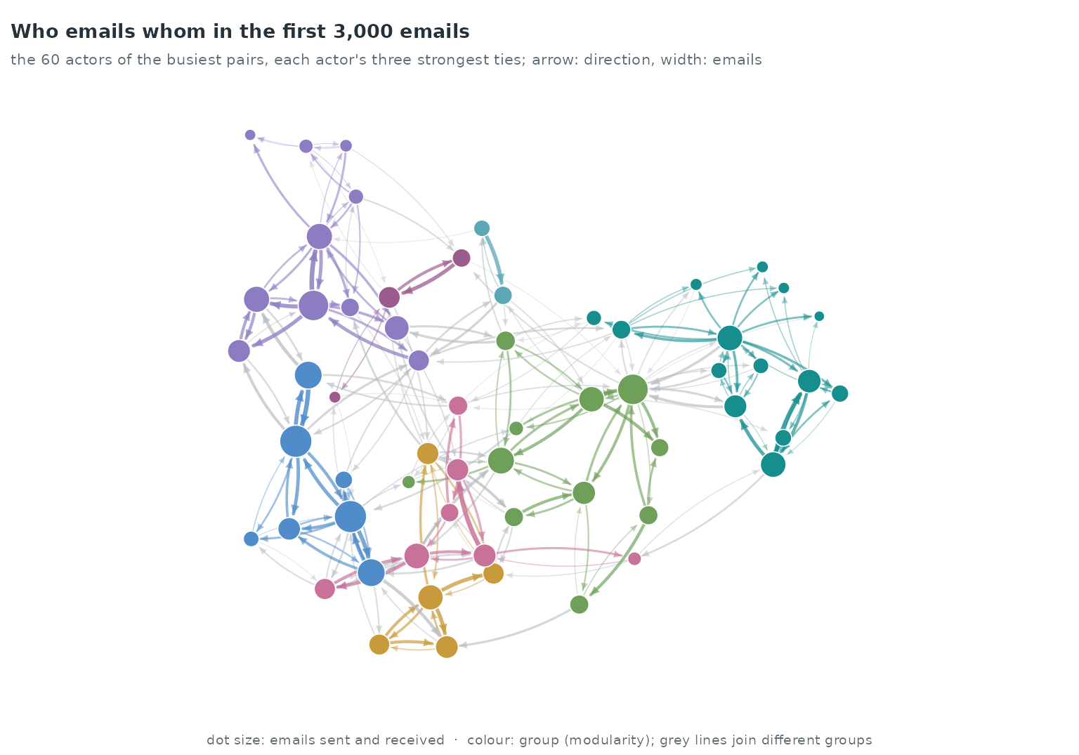

The animation covers the whole log, 12,216 emails over 802 days, two weeks per frame; the analysis below uses its first 3,000 emails, which end on day 158. 18 of the 58 windows have no email, and the busiest, days 196–210, has 584.

The strata are split in time: the first 80% of the emails train the models, the last 20% are held out.

cut   <- stats::quantile(unique(feat$stratum), 0.8)
train <- feat[feat$stratum <= cut, ]
test  <- feat[feat$stratum >  cut, ]
c(train_events = length(unique(train$stratum)),
  test_events  = length(unique(test$stratum)))
#> train_events  test_events 
#>         2400          600

fm <- event ~ reciprocity_count + transitivity_count + sender_outdegree +
  receiver_indegree + recency

Conditional logistic regression

fit_cl <- rem(fm, data = train, method = "clogit", stratum = "stratum")
round(summary(fit_cl)$coefficients[, c("coef", "se(coef)", "z")], 3)
#>                     coef se(coef)      z
#> reciprocity_count  1.136    0.081 14.087
#> transitivity_count 0.729    0.096  7.611
#> sender_outdegree   0.419    0.042 10.090
#> receiver_indegree  0.280    0.048  5.797
#> recency            3.459    0.199 17.352

Neural backends

method = "nn" trains on the same partial likelihood. A fraction of the training strata (validation = 0.2) is held back for early stopping. nn_control() selects the architecture: a multilayer perceptron scores the five statistics jointly, while architecture = "additive_spline" fits one B-spline curve per statistic and adds them.

fit_mlp <- rem(fm, data = train, method = "nn", stratum = "stratum",
               nn = nn_control(hidden = c(16, 8), epochs = 150,
                               patience = 10, seed = 1))
fit_add <- rem(fm, data = train, method = "nn", stratum = "stratum",
               nn = nn_control(architecture = "additive_spline", spline_df = 8,
                               epochs = 300, seed = 1))
fit_mlp$fit
#> Neural conditional-logistic REM fit
#>   architecture : 5 - 16 - 8 - 1  (relu)
#>   parameters   : 241
#>   strata       : 2400
#>   best epoch   : 39
#>   val concord. : 0.846
fit_add$fit
#> Neural conditional-logistic REM fit
#>   architecture : additive B-splines (df = 8 per feature, 5 features)
#>   parameters   : 41
#>   strata       : 2400
#>   best epoch   : 300
#>   val concord. : 0.832

The perceptron stopped at epoch 39; the spline model’s best validation loss was at epoch 300 of the 300 allowed, so its training stopped at the epoch limit rather than by early stopping.

Held-out comparison

On the held-out emails each model scores the event and its three controls. The table reports the share of strata in which the event gets the highest score (ties split evenly), and the mean log partial likelihood per held-out event. A model that ignores the covariates ranks the event first in one stratum out of four.

score_clogit <- function(d) as.vector(as.matrix(d[, stats]) %*% coef(fit_cl))
scores <- list(clogit          = score_clogit(test),
               nn_mlp          = predict(fit_mlp$fit, test),
               nn_spline       = predict(fit_add$fit, test))

rank_first <- function(sc, d) mean(tapply(seq_len(nrow(d)), d$stratum, function(ix) {
  s <- sc[ix]; e <- d$event[ix] == 1
  if (s[e] < max(s)) 0 else 1 / sum(s == max(s))
}))
log_pl <- function(sc, d) mean(tapply(seq_len(nrow(d)), d$stratum, function(ix) {
  s <- sc[ix]; s[d$event[ix] == 1] - (max(s) + log(sum(exp(s - max(s)))))
}))
held_out <- data.frame(
  model          = names(scores),
  event_ranked_1 = vapply(scores, rank_first, 0, d = test),
  mean_log_pl    = vapply(scores, log_pl, 0, d = test))
knitr::kable(held_out, digits = 3, row.names = FALSE)

model	event_ranked_1	mean_log_pl
clogit	0.817	-0.531
nn_mlp	0.808	-0.544
nn_spline	0.823	-0.521

All three models rank the held-out event first in between 0.808 and 0.823 of the strata, against 0.25 for a model without covariates. The highest mean log partial likelihood on the held-out emails is that of nn_spline.

Effect curves

Each panel varies one statistic over its 1st–99th percentile range with the other four at their training means, and shows the change in score centred at its mean over the range: the straight line of the conditional logit and the partial-dependence curves of the two neural models.

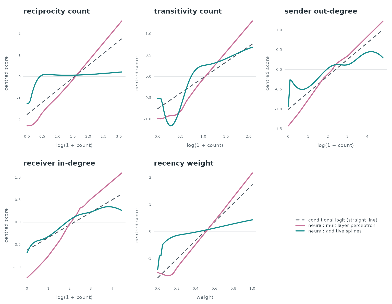
Between the 1st and the 99th percentile the score increases for 5 of the 5 statistics under the conditional logit, 5 under the perceptron and 5 under the spline model. The spline curves change most over the lowest values, where many rows share the value 0 (a dyad, sender or receiver with no earlier email of that kind), and some have kinks there: the B-spline knots are placed at quantiles of the feature, and with many tied values several knots fall close together.

Bootstrap bands for the neural model

The neural backend has no coefficient table. nn_uncertainty() resamples the training strata with replacement, refits the network on each resample with the same nn_control() settings, and returns pointwise bands for the centred partial-dependence curves and an interval for the in-sample concordance. Fifteen resamples keep the page quick to build; the bands are coarse at that number.

unc <- nn_uncertainty(fit_mlp, data = train, stratum = "stratum", B = 15,
                      seed = 1)
unc
#> Bootstrap uncertainty for a neural rem() fit
#>   resamples    : 15 (15 successful)
#>   level        : 95%
#>   features     : reciprocity_count, transitivity_count, sender_outdegree, receiver_indegree, recency
#>   concordance  : 0.835  [0.807, 0.841]
#> Use plot() for per-feature partial-dependence bands.

plot(unc)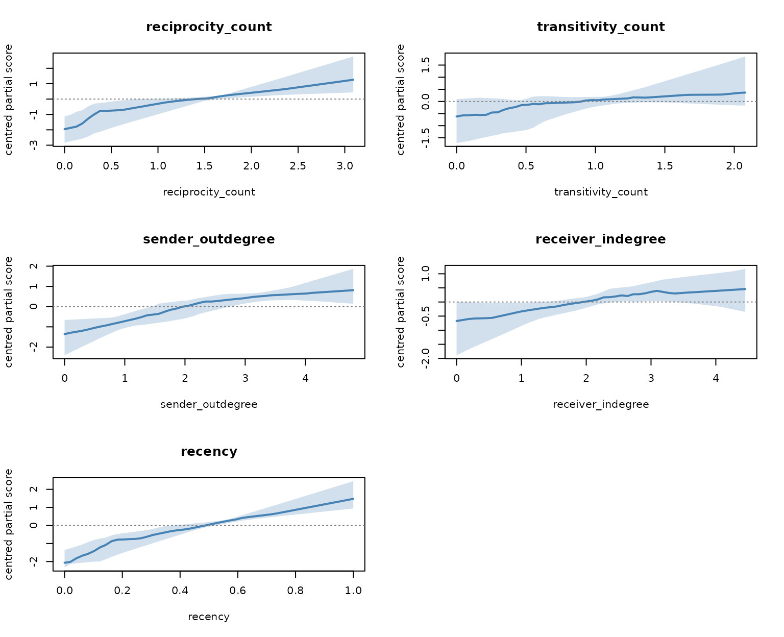

nn_uncertainty() evaluates each curve from the 1st to the 99th percentile of the feature, with the other features at their means.

Time-varying effects with the gam backend

The gam backend fits a case-1-control design, so a new sample with one control per email is drawn and widened to one row per email. tv(x) lets the effect of x change smoothly over time; tvnl(x) lets it change in both time and the value of x (a tensor-product smooth). Both are compared with the model that holds the two effects constant.

cc1  <- sample_non_events(eu, n_controls = 1, seed = 2)
f1   <- endogenous_features(cc1, stats = c("reciprocity_count", "transitivity_count"))
for (s in c("reciprocity_count", "transitivity_count")) f1[[s]] <- log1p(f1[[s]])
wide <- widen_case_control(f1, covariates = c("reciprocity_count",
                                              "transitivity_count", "time"))

fit_const <- rem(~ reciprocity_count + transitivity_count, data = wide,
                 method = "gam")
fit_tv    <- rem(~ tv(reciprocity_count, k = 6) +
                   tvnl(transitivity_count, k = c(5, 5)),
                 data = wide, method = "gam", time = "time")
aic <- c(constant = AIC(fit_const$fit), time_varying = AIC(fit_tv$fit))
round(aic, 1)
#>     constant time_varying 
#>       1849.4       1813.4
summary(fit_tv)$s.table
#>                                      edf   Ref.df   Chi.sq p-value
#> s(.time):reciprocity_count      2.912997 3.371272 372.4179       0
#> te(.T,.X_transitivity_count):.I 6.441087 7.716032 322.0352       0

The time-varying model’s AIC is 36.1 lower than that of the constant-effect model.

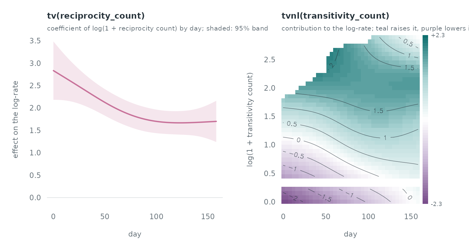
In the left panel the coefficient of reciprocity_count is 2.83 on day 0 and 1.70 on day 158; the band is a 95% interval. The right panel shows the tensor-product surface of tvnl(transitivity_count) over day and count; mgcv leaves blank the combinations of day and count with no data near them, which includes the gap between a count of 0 and a count of 1 on the log1p() scale.