Case study: armed-conflict dyads, 1946

Armed-conflict dyads, 1946–2025

ucdp_dyads is the dyadic dataset of the Uppsala Conflict Data Program (UCDP, version 26.1, CC BY 4.0): one row for every year in which a government (sender, side A) and an opponent (receiver, side B) fought with at least 25 battle-related deaths. The opponent is a rebel group, or another government in an interstate conflict. intensity_level is 2 (war, 1,000 or more deaths in the year) or 1 (minor conflict). This case study asks how strongly a dyad’s own past predicts its fighting in a given year, how fast that memory fades once a conflict stops, and whether a government at war with one opponent is more likely to fight another.

data(ucdp_dyads)
u <- ucdp_dyads
c(dyad_years = nrow(u), dyads = length(unique(u$dyad_id)),
  governments = length(unique(u$sender)), opponents = length(unique(u$receiver)),
  first = min(u$year), last = max(u$year))
#>  dyad_years       dyads governments   opponents       first        last 
#>        3518         697         121         614        1946        2025
table(type = type_lab[as.character(u$type_of_conflict)], intensity = u$intensity_level)
#>                               intensity
#> type                              1    2
#>   extrasystemic                 105   29
#>   internationalized intrastate  436  253
#>   interstate                     96   59
#>   intrastate                   2148  392

A few sides are coalitions (side A lists several governments, for example the Arab states in 1948); each is kept as one actor.

Who fights whom

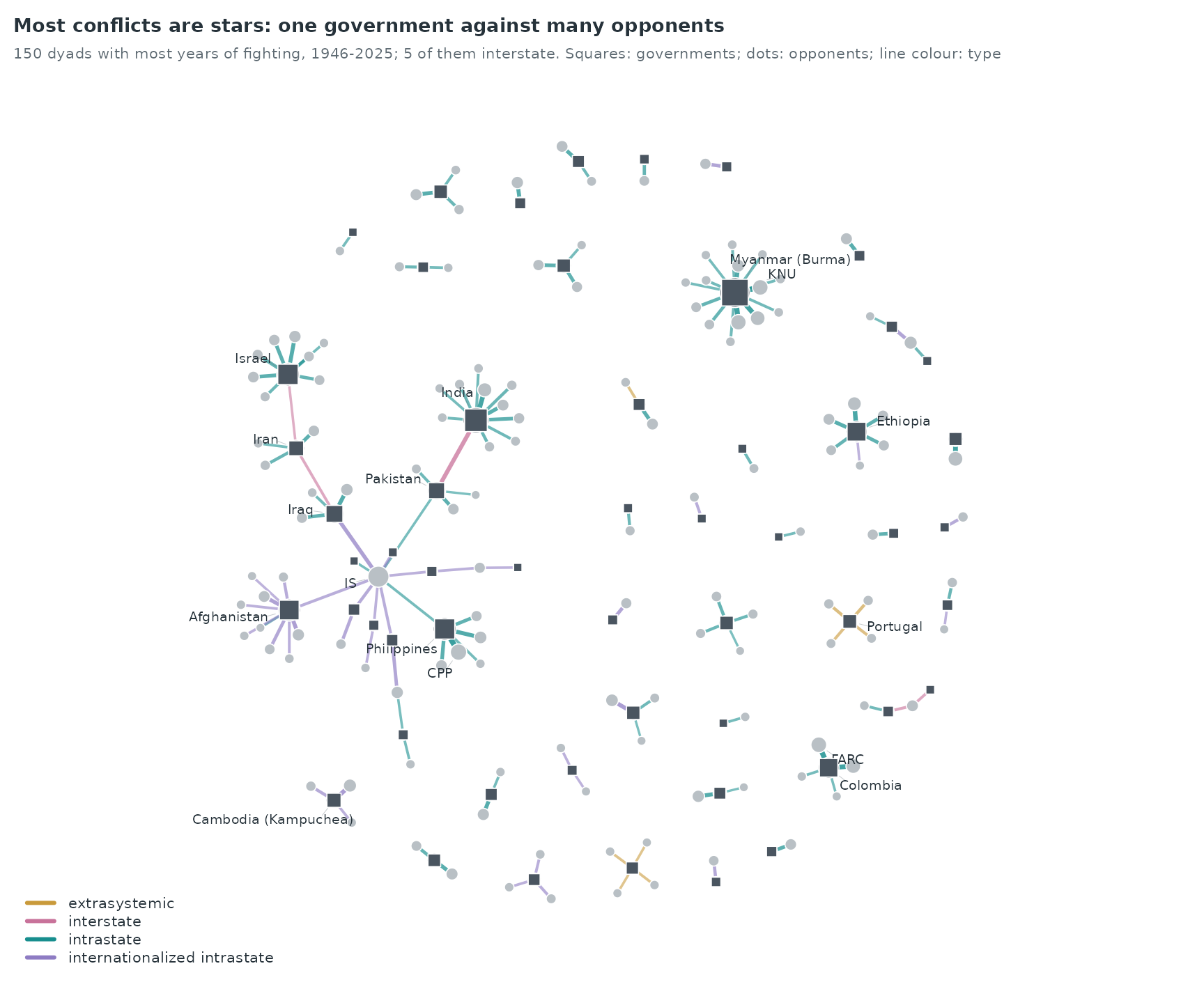
Network of governments and their opponents for the dyads with the most years of fighting, coloured by type of conflict

Intrastate conflicts make the network a set of stars: one government against many rebel groups. Myanmar (Burma) has fought 43 different opponents, Chad 30 and India 28. Interstate dyads join governments to each other and appear as the few lines between stars.

Spells, gaps and recurrence

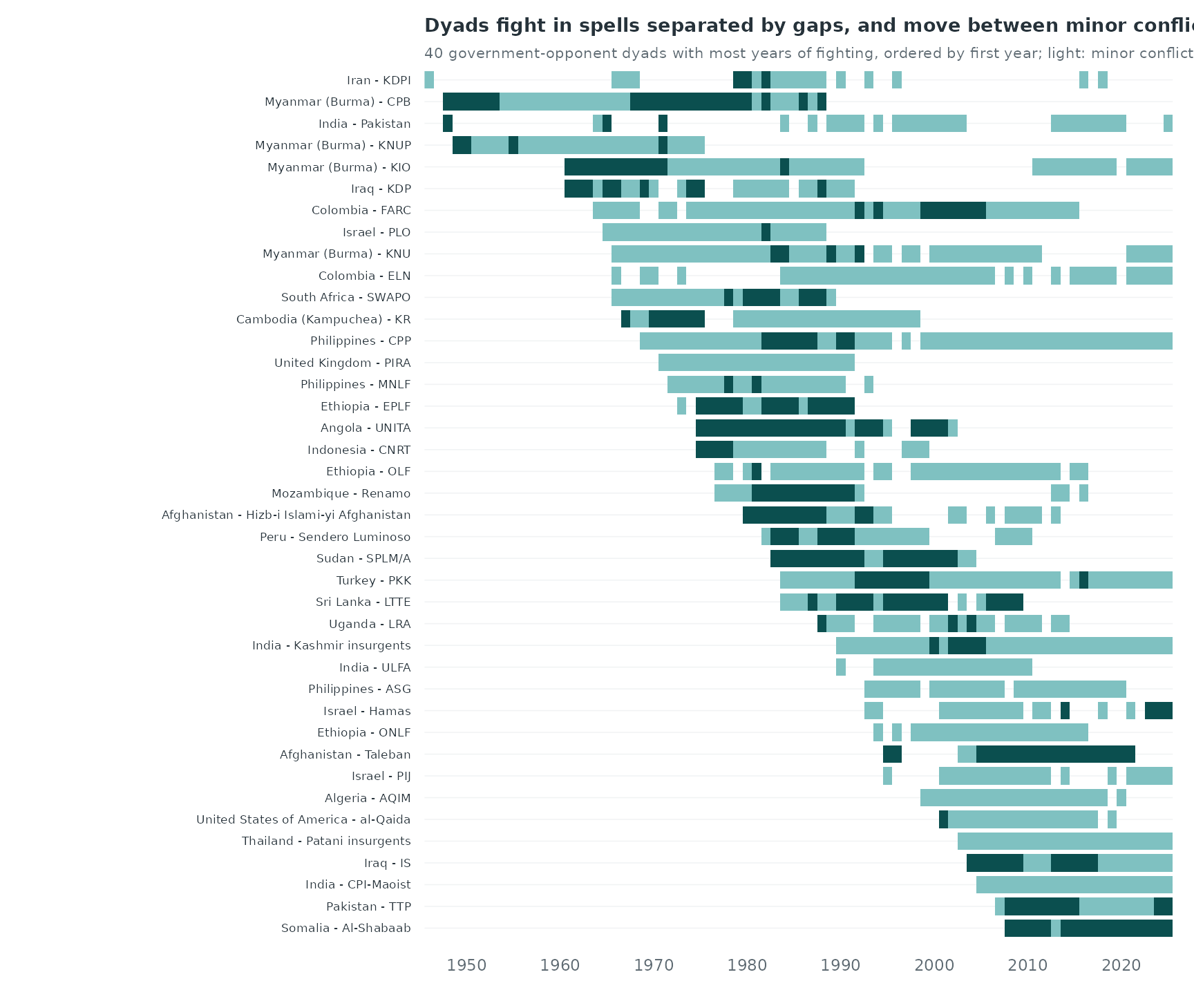
One row per dyad and one column per year, coloured by intensity, for the 40 dyads with the most years of fighting

The number of dyads that fight within a two-year window is 22 in 1946-1947, peaks at 91 in 1990-1991, and is 87 in 2024-2025.

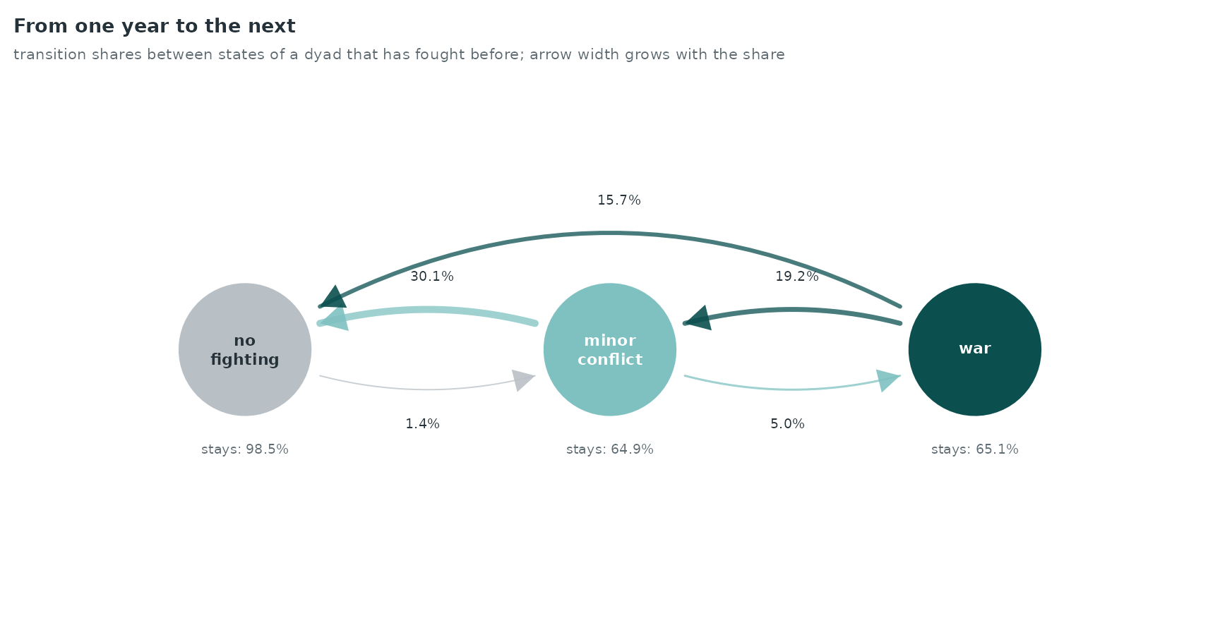
Most long dyads fight in spells: years of fighting, a gap, and fighting again with the same opponent. The next figure counts how often a dyad that has fought before is active again, by the number of years since it last fought.

active <- split(u$year, paste(u$sender, u$receiver, sep = "\r"))
haz <- do.call(rbind, lapply(active, function(y) {
  y <- sort(unique(y)); yrs <- (min(y) + 1):2025
  last <- vapply(yrs, function(t) max(y[y < t]), 0)
  data.frame(gap = yrs - last, active = yrs %in% y)
}))
h <- aggregate(list(active = haz$active, n = rep(1, nrow(haz))), list(gap = haz$gap), sum)
h$rate <- h$active / h$n
head(h, 4)
#>   gap active    n       rate
#> 1   1   2508 3450 0.72695652
#> 2   2    133  923 0.14409534
#> 3   3     57  781 0.07298335
#> 4   4     39  711 0.05485232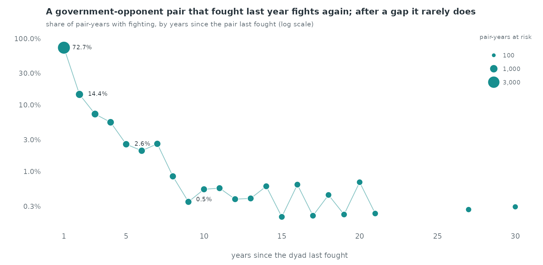

Share of dyads fighting again, by years since they last fought

A dyad that fought last year fights again with probability 72.7%. After a gap of two years the share is 14.4%, after five years 2.6% and after ten years 0.5%.

Escalation and de-escalation

Diagram of yearly transitions between peace, minor conflict and war for dyads that have fought before

A minor conflict becomes a war the next year in 5.0% of cases; a war stays a war in 65.1% and drops to a minor conflict in 19.2%.

Case-control design for yearly events

The events are dyad-years: (government, opponent, year). All events of a year share the same time, which matters for both the controls and the statistics.

Risk set. The question is which of the dyads that have fought before is active in a given year. sample_non_events(mode = "two") would draw controls from every government × opponent pair, and most of those pairs never could fight (a government and a rebel group of another continent); the dyad’s own past would then separate events from controls almost perfectly. The controls are therefore drawn from the dyads that fought in an earlier year: five per event, uniformly, excluding the event’s own dyad. A dyad’s first year (its onset) has no comparable risk set here and is left out. A control may be a dyad that also fought in the same year, as another row: this is the Breslow convention for tied times, which keeps a tied event at risk.

ev <- u[order(u$year, u$dyad_id), ]
el <- data.frame(sender = ev$sender, receiver = ev$receiver, time = ev$year)
dk <- paste(el$sender, el$receiver, sep = "\r")
first_year <- tapply(el$time, dk, min)
set.seed(1)
cc <- do.call(rbind, lapply(which(el$time > first_year[dk]), function(i) {
  pool <- setdiff(names(first_year)[first_year < el$time[i]], dk[i])
  sr <- do.call(rbind, strsplit(sample(pool, 5), "\r"))
  data.frame(stratum = i, event = c(1L, rep(0L, 5)), sender = c(el$sender[i], sr[, 1]),
             receiver = c(el$receiver[i], sr[, 2]), time = el$time[i])
}))
c(strata = length(unique(cc$stratum)), rows = nrow(cc), onsets_left_out = sum(el$time == first_year[dk]))
#>          strata            rows onsets_left_out 
#>            2823           16938             695

Statistics. endogenous_features() updates the history row by row, so an event would see the other rows of its own year. To use only earlier years, each year’s rows are scored with prior_log holding the events of all earlier years and an empty history_log, so no row of the current year enters the history.

yrs <- sort(unique(cc$time))
cc <- do.call(rbind, lapply(yrs, function(y)
  endogenous_features(cc[cc$time == y, ], history_log = el[0, ],
                      prior_log = if (any(el$time < y)) el[el$time < y, ],
                      stats = c("recency", "sender_outdegree", "receiver_indegree"))))
# the dyad's own past: number of earlier active years, and war last year
dkey <- dk; ckey <- paste(cc$sender, cc$receiver, sep = "\r")
cc$dyad_past <- mapply(function(k, t) sum(dkey == k & el$time < t), ckey, cc$time)
war_key <- paste(dkey, el$time)[ev$intensity_level == 2]
cc$war_last <- as.numeric(paste(ckey, cc$time - 1) %in% war_key)
cc$last_year <- as.numeric(!is.na(cc$recency) & cc$recency == 1)
# the government's other dyads active last year
gov_last <- table(paste(el$sender, el$time))
cc$gov_other <- as.numeric(gov_last[paste(cc$sender, cc$time - 1)]); cc$gov_other[is.na(cc$gov_other)] <- 0
cc$gov_other <- cc$gov_other - cc$last_year
cc$log_dyad_past <- log1p(cc$dyad_past)
cc$log_gov_past <- log1p(cc$sender_outdegree); cc$log_opp_past <- log1p(cc$receiver_indegree)
cc$log_gov_other <- log1p(cc$gov_other)

Linear model

covs <- c("last_year", "war_last", "log_dyad_past", "log_gov_other", "log_gov_past", "log_opp_past")
fit <- rem(reformulate(covs, response = "event"), data = cc, method = "clogit")
ct <- summary(fit$fit)$coefficients
round(ct[, c("coef", "exp(coef)", "se(coef)")], 2)
#>               coef exp(coef) se(coef)
#> last_year     3.68     39.57     0.09
#> war_last      0.03      1.03     0.08
#> log_dyad_past 0.14      1.15     0.07
#> log_gov_other 0.07      1.07     0.06
#> log_gov_past  0.05      1.05     0.04
#> log_opp_past  0.18      1.19     0.06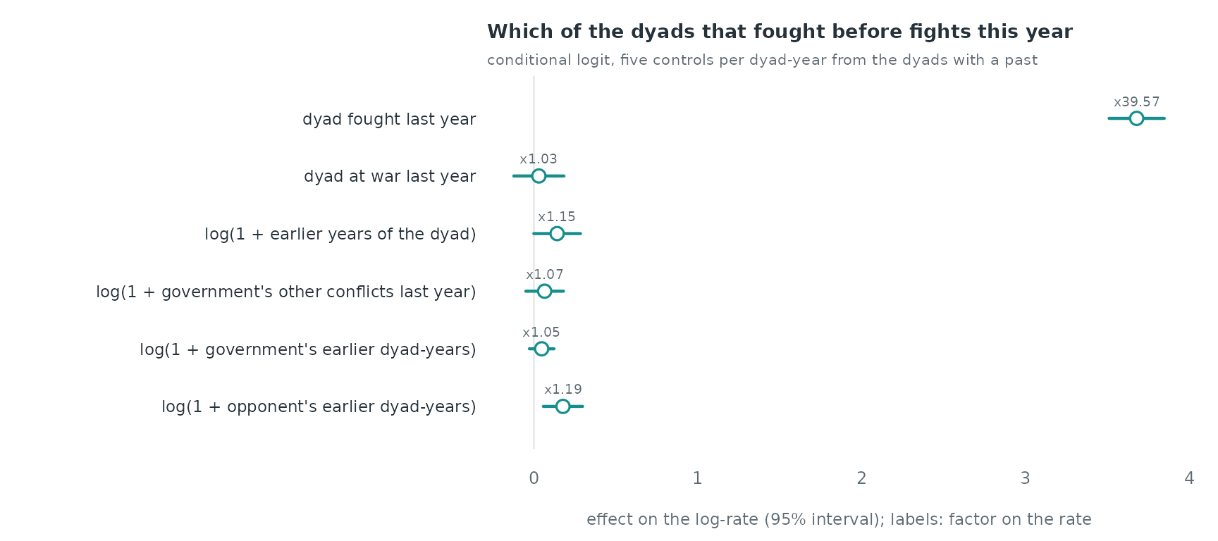

Coefficients of the conditional logit with 95% intervals

Fighting last year multiplies the rate by 39.6, holding the other terms fixed, and war last year by a further 1.0. Each unit of log(1 + earlier years) of the dyad multiplies it by 1.2. The government’s other conflicts last year multiply the rate of fighting a given opponent by 1.1 per unit, and its total earlier dyad-years by 1.0.

How fast the memory of a conflict fades

The recurrence shares above do not separate the gap from the other terms. In the gam backend (one control per dyad-year) the gap enters as a smooth nl() of the log of the years since the dyad last fought; a gap of one year is “fought last year”, so the smooth replaces that indicator. tv() lets the effect of the government’s other conflicts change over the eighty years.

cc$gap <- log(cc$recency)
cc$year <- cc$time
w <- widen_case_control(cc, covariates = c("gap", "war_last", "log_gov_other", "log_opp_past", "year"))
gfit <- rem(~ war_last + log_opp_past + nl(gap, k = 6) + tv(log_gov_other, k = 6),
            data = w, method = "gam", time = "year")
summary(gfit)$s.table
#>                             edf   Ref.df      Chi.sq   p-value
#> s(.X_gap):.I           1.000296 1.000592 345.9482902 0.0000000
#> s(.time):log_gov_other 2.000748 2.001496   0.8116265 0.6667807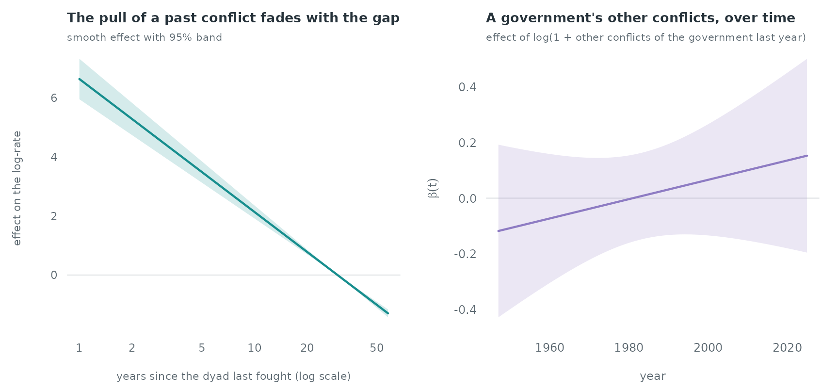

Smooth effect of years since the dyad last fought, and the time-varying effect of the government's other conflicts

The fitted smooth is close to a straight line in the log of the gap (1.0 effective degrees of freedom), so the rate falls as a power of the gap, about gap^-2.0. On the log-rate scale it falls by 4.50 between a dyad that fought one year ago and one that last fought ten years ago, a factor of 90 on the rate. The effect of the government’s other conflicts is -0.07 around 1960, 0.03 around 1990 and 0.14 around 2020 (log-rate per unit of log(1 + conflicts)); the test of the time-varying term gives p = 0.67, so the data do not show a change over time.

What the design leaves out

Onset of new dyads. First years of dyads are left out; the model describes which dyads with a past fight again, not how new conflicts start.
Deaths. The data give only the intensity class; the number of deaths is in the UCDP battle-related deaths dataset.
Global trends (the end of the Cold War, the year itself) cancel within a stratum, since every row of a stratum has the same year; tv() above captures how an effect changes, not how the overall number of conflicts changes.

Case study: armed-conflict dyads, 1946–2025