ED: evolutionary distinctiveness, raw and centred
In one line. \(\mathrm{ED}_s(t)\) is the share of the clade's phylogenetic diversity that lineage \(s\) alone represents, and its coefficient asks whether being distinct changes what a lineage does next: the relict question of the EDGE programme turned round.
\(\mathrm{ED}\) is a lineage-level covariate read along the whole path from the crown to the lineage. The package offers it raw, in ed and ned, and centred on its clade mean, in edc and nedc. It shares its last term, the pendant edge, with D, and on unbalanced trees it ranks lineages in partly the same order as K; the covariates page compares the four.
The question in the literature
Evolutionary distinctiveness was built for conservation, not for diversification. Vane-Wright et al. (1991) asked which species to protect when not all can be, and Faith (1992) defined phylogenetic diversity (PD) as the total branch length a set of species spans. The per-species apportionment of that length followed, as equal splits and as fair proportion (Redding and Mooers 2006; Isaac et al. 2007); fair proportion is the ED of the EDGE lists. It divides every branch on a species' path from the root equally among the living species below it, so a species with few close relatives, or a long terminal branch, carries a large share, and the shares sum to Faith's PD. Redding et al. (2008) showed that ranking by it captures more PD than the same number of random species, and Steel et al. (2007) gave the expected contribution of a species under extinction risk. Redding et al. (2014) compared eleven isolation metrics; Tucker et al. (2017) placed them in a common framework; Gumbs et al. (2023) revised the EDGE protocol on the same quantity. In birds, Jetz et al. (2014) found ED distributed very unevenly over the tree.
Reading ED as a diversification covariate asks not what would be lost if a distinct lineage died, but whether being distinct changes the lineage's rates. Two positions exist under the names relict and living fossil. On the dead-end view a distinct lineage is the survivor of a group that has been losing members, alone because its relatives are gone and on the way out itself; Purvis et al. (2000) and Heard and Mooers (2000) showed that extinction concentrated on such lineages removes more history than random extinction would. On the panchronic view a distinct lineage persists through epochs at low rates of both speciation and extinction. Bennett et al. (2017) simulated trees in which both rates were functions of tip ED with random signs and found that the trees closest in shape to empirical ones were those in which the most distinct tips had lower rates of both: the panchronic reading fitted and the dead-end one did not. Grandcolas et al. (2014) argued that the relict concept conflates a phylogenetic, a biogeographic and a morphological property. The published model closest to the ED models is that of Qin et al. (2025), in which speciation depends on evolutionary relatedness measured at scales from the nearest neighbour to the whole clade; it is simulation-only, with a neural-network estimator proposed since (Qin et al. 2026).
What the package computes
Fair proportion on the complete tree at time \(t\):
\[ \mathrm{ED}_s(t) = \sum_{b \succeq s} \frac{\ell_b(t)}{n_b(t)}, \qquad \sum_{s \in A(t)} \mathrm{ED}_s(t) = \mathrm{PD}(t), \]
where \(b\) runs over the branches from the crown to \(s\), \(\ell_b(t)\) is the length of branch \(b\) up to \(t\) and \(n_b(t)\) the number of lineages alive at \(t\) that descend from it. The last branch on the path has one descendant, \(s\) itself, and contributes the pendant age \(E_s(t)\); the rest is the ancestral share \(A_s = \mathrm{ED}_s - E_s\). ED has units of time.
When it changes. Between two events every ancestral share is constant and only the pendant edge grows, so raw \(\mathrm{ED}_s(u) = c_s + (u - \tau_s)\) rises at slope one for every lineage alive, with \(c_s\) the constant that one pass over the tree returns (inst/include/ed_covariate.hpp, shared by the simulator and the likelihood). At an event it jumps. A split anywhere below a branch \(b\) raises \(n_b\) and lowers the share of \(b\) for every relative that descends from it; a death lowers \(n_b\) and raises those shares. The lineage that splits loses most: its former pendant edge is now shared by two. Hidden events count in both directions, so an extinct sister lowers a living lineage's ED while it lives and raises it when it dies.
Raw and centred. The clade mean of raw ED is \(\mathrm{PD}/N\), phylogenetic diversity per lineage, a clade-level quantity that rises with the clade's age and falls with its diversity. In ed and ned the coefficient \(\beta_{ED}\) therefore carries a clade-level component and a within-clade contrast at once. The centred covariate
\[ \mathrm{ED}^c_s(t) = \mathrm{ED}_s(t) - \frac{\mathrm{PD}(t)}{N(t)} \]
sums to zero and keeps the contrast only; because every \(\mathrm{ED}_s\) grows at the same unit rate, \(\mathrm{ED}^c_s\) is constant on a segment. edc reduces to cr on a clade whose lineages are equally distinct, and nedc to dd at \(\beta_{ED} = 0\). An ED model needs a phylo object and refuses a bare vector of branching times.
What the sign of a coefficient means
Speciation. A negative \(\beta_{ED}\) says that distinct lineages speciate less: the panchronic direction on the speciation side, persistence at a low rate. A positive \(\beta_{ED}\) says that distinct lineages speciate more, the direction the relatedness mechanism of Qin et al. (2025) predicts if competition among close relatives is what limits speciation, since a lineage with few close relatives has less of it; it is also the direction in which isolation in the tree stands for unoccupied space around the lineage.
Extinction. A negative \(\gamma_{ED}\) is the panchronic view, distinct lineages persisting; a positive one is the dead-end view.
What else produces the same sign. ED is retrospective. At the tips, fair proportion and equal splits are close to the inverse of the DR statistic, which Title and Rabosky (2019) showed tracks the speciation rate of a lineage's recent ancestry. A lineage is distinct because its ancestry speciated slowly, and if rates are inherited its ancestry's slow rate is its own: a negative \(\beta_{ED}\) is then rate persistence, not an effect of distinctiveness, and the two are the same statement about the tree with different words for the cause. On raw ED, the clade-level part \(\mathrm{PD}/N\) lets a fit match a time trend in the clade's rate through \(\beta_{ED}\), which is the one way a tree with no lineage-level effect can produce a spurious raw-ED selection. Because ED is read on the complete tree, its value depends on the extinction rate through the hidden lineages drawn, so the ED coefficients and the extinction rate are not independent in a fit.
What ED cannot be separated from
D, through the shared pendant edge. \(\mathrm{ED}_s = E_s + A_s\), and \(D_s\) is \(E_s\) centred. Within one tree over the lineages alive at three times, the rank correlation of \(D\) and ED is 0.57 on simulated dd clades, 0.62 on the same clades reconstructed and 0.74 on the 47 family trees (E39); ED and the nearest-neighbour distance correlate at 0.87 to 0.88. On the covariate path a generator with both effects returns \(D\) alone on 0.80 of trees at 100 tips (E20), and on ned trees \(D\) replaces ED as the first covariate as trees grow, 19 of 20 at 400 tips (E22). The question that would separate them, whether the ancestral share \(A_s\) matters, needs a covariate the package does not offer.
K, on unbalanced trees. A lineage deep in a radiation has many ancestral splits and a small share of every branch it sits on; a lineage alone on a long branch has few splits and a large share. On simulated trees the two are nearly separate within a tree (median ED-K rank correlation \(-0.11\) complete, \(-0.18\) reconstructed), on the 47 family trees they are not (median \(-0.44\), as far as \(-0.84\)), and the tie grows with imbalance: across families the rank correlation of the Colless index with the ED-K correlation is \(-0.51\) (E39). On trees generated with a \(K\) effect, ED enters the path first, on every tree, carrying the \(K\) signal with the sign reversed (E21).
Its own intercept. Raw ED grows with time like its clade mean, so on a single tree \(\beta_0\) and \(\beta_{ED}\) lie on a ridge. On complete 100-tip trees, where nothing is hidden, the per-tree maximum places them along it (\(\beta_{ED}\) at 0.81 and 1.22 of its value at \(\mp 0.35\)), while the pooled maximum over 261 and 348 trees returns 1.005 and 1.002; centring removes the ridge, and edc and nedc return 1.04, 1.07, 1.03 and 1.01 (E44).
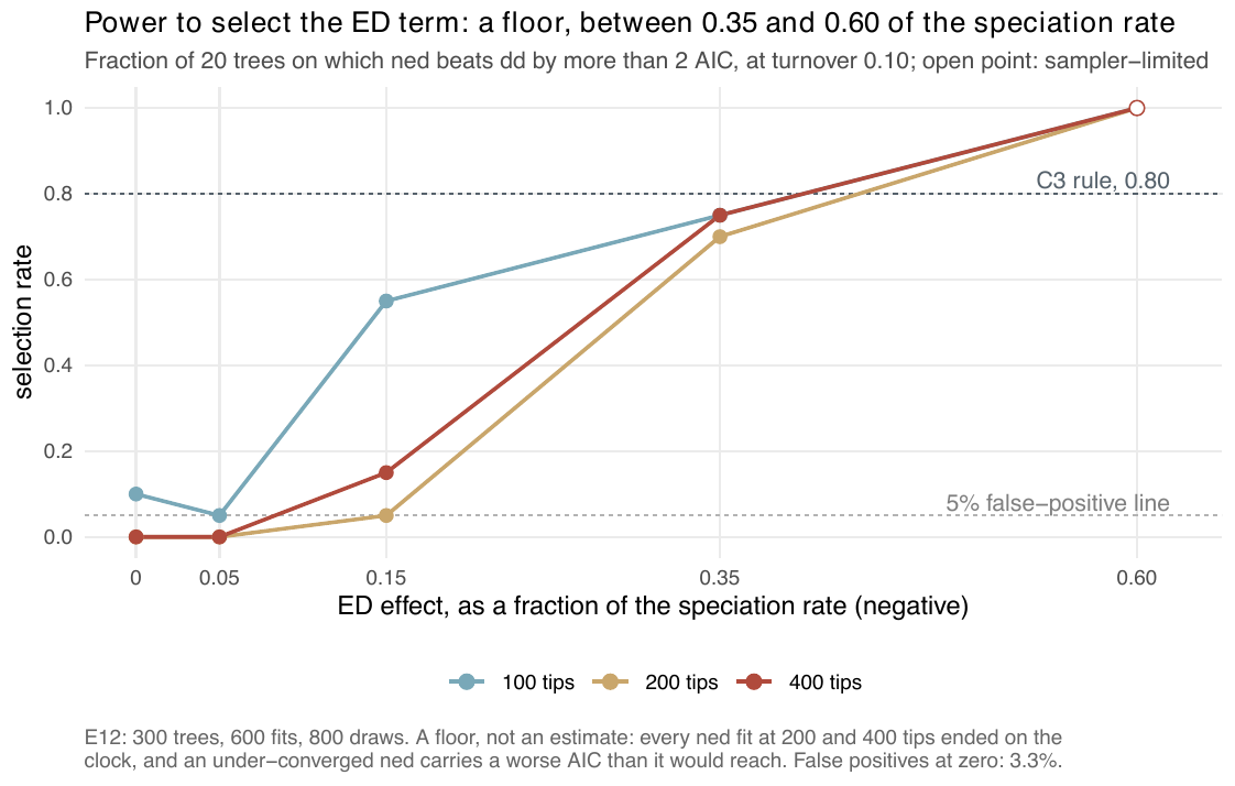
ned beats dd by more than 2 AIC, at turnover 0.10 on the linear link, by the ED effect as a fraction of the speciation rate per clade-mean unit of ED. Every ned fit at 200 and 400 tips ended on its clock, so the curves are floors. The trees were simulated before the \(\mathrm{ED}\) simulator correction of f30a791; V7 measures selection under the conditioned likelihood. From E12.What simulation says
ED is the lineage-level coefficient the estimator recovers best.
- Sign. The sign of \(\beta_{ED}\) is recovered on at least 0.95 of trees at every effect of 0.15 of the speciation rate and stronger, at 100, 200 and 400 tips, on linear-link trees simulated before
f30a791(E12). Conditioned on survival, on the exponential link and the current simulator, at 50 and 100 tips and \(\pm 0.35\) per scale unit, the sign is right on 92% to 100% ofed,edcandnedcfits and on 77% and 93% ofnedfits at turnover 0.10 (V5, interim). - Size. On unfinished fits the size is attenuated (0.69, 0.40 and 0.19 of its value at \(-0.60\) from 100 to 400 tips) and comes back with more iterations (0.96, 0.67 and 0.72 at \(-0.35\) with 300 iterations) (E12, on the same pre-
f30a791trees); on the 7 fits that met the stopping rule at 200 tips it is 1.02 (E29). Under the exact simulator,edalone returns 0.85 and 1.10 at \(\mp 0.35\) (E24, part b), andedc0.96 and 1.02 with the right sign on every tree (E24). - Selection. Selecting
nedoverddon 0.80 of trees needs an effect between \(-0.35\) and \(-0.60\) of the speciation rate, at 100 to 400 tips and at turnover 0.10 and 0.25 (Figure 1; E12, E16). At \(-0.15\) selection is 0.05 to 0.55, and centring does not lift it (0.10 to 0.20; E18); these cells ran on trees simulated beforef30a791; conditioned on survival,nedis chosen on 1 of 19 of its own trees at \(\pm 0.35\) and 100 tips (V7).edcis selected overcron 0.95 and 0.85 of trees at \(\mp 0.35\) (E24). In the one-call ladder, read by the parsimonious rule,nedis chosen on at most 2 of 20 of its own trees in any condition of E27, although its coefficient is recovered at 0.91 to 0.98 in three of them: the two extra parameters are not paid for at these sizes (unconditioned fits, mostly ended by the clock; V5 and V7 remeasure them conditioned on survival). - False positives. On trees with no lineage-level effect,
nedis selected on 2 of 60 (E12) and 0 of 15 (E16);edc,nedcandedon 0 to 1 of 20 (E18, E24); on trees from another group's simulator, on 0.05 and 0.00 (E11). - Where it breaks. On an early build, with the linear link and trees simulated before
f30a791,nedestimates at turnover 0.5 were biased by 1 to 4 standard deviations and trees with no ED effect selectednedon up to 0.9 of them; at \(\rho = 0.7\) the effective sample fell below 10 outside the weakest effects (E2). V5 measures turnover and V6 the sampling fraction on the current build. - Extinction. The extinction slope on ED, generated at zero, is fitted at \(-0.25\) to \(-0.73\) per unit in every
edcell (E24), and at 200 tips it is returned on the lower limit of the box whatever its generating value (E29, E32). Where the generating brake on speciation is strong, the fit adds a brake on extinction the generator did not have, so a negative \(\gamma_{ED}\) on a real clade has a known way of arising from nothing.
What real phylogenies say
The 46 family trees. Under the parsimonious rule ned is the choice in 6 of the 24 families of the calibrated range whose minimum-AIC fit is readable (E28), and by minimum AIC, the sensitivity reading, in 6 there too. The parsimonious reading was fixed before the data, and Monte Carlo EM log-likelihoods carry Monte Carlo error and a downward bias, so a difference below 2 AIC is within the estimator's noise. In the merged 46-family table, ned leads dd by more than 2 AIC in 15 families and is the minimum-AIC lineage-level winner in 6 (E26). \(\beta_{ED}\) is negative in 29 of the 31 ned fits with at least 10 effective draws, with a median speciation factor of 0.69 per standard deviation of ED (0.33 to 1.08). Four of those six ned families have a \(\gamma\) statistic between \(-5.9\) and \(-7.7\), below every family in which nk is chosen. In the New World warblers (Parulidae) ned leads dd by 24 AIC with a factor of 0.40: the fast lineages are the yellowthroats of Geothlypis and part of Setophaga, the slowest the ovenbird, the worm-eating warbler and the black-and-white warbler, each the only species of its genus on a branch that reaches back near the base of the family. Where the ladder chooses ned, the covariate path keeps ED in all 6 families.
The 170 bird and mammal trees. ned is the parsimonious choice on 50 trees. The ED factor is below 1 on all 45 readable chosen fits, median 0.49 per standard deviation, and on 141 of 145 readable ned fits whether chosen or not, median 0.62. 31 of those \(\beta_{ED}\) values end on the lower edge of the box, so their factors are the box's bound and not the tree's. The ED factor falls with the tree's Colless imbalance (rank correlation \(-0.57\) over 145 fits). On pairs of trees of the same taxon, a clade cut from a class tree and its family tree, the factor is below 1 on both members on 10 of 10 (E40, Real phylogenies).
How to read it. Distinct lineages speciate less, wherever the model is chosen. That is the sign the EDGE literature assumes when it treats the distinct species of a clade as relicts, and also the sign of an inherited low rate and of the \(K\) effect read from the other end of the tree: where both ned and nk rest on at least 10 effective draws on a family, nk has the lower AIC in 19 of 25, by a median 3.6 units, and the lineages a distinctiveness ranking puts first (the ovenbird, the bobolink, the crested jay) are those the fitted models give the lowest speciation rates.
Not yet read.
- The extinction side. On every real tree the ED slope on extinction sits on a box edge, and the exact constant-rate likelihood excludes zero extinction on none of the 16 smallest trees tested (E41), so the half of the panchronic hypothesis that separates it from rate persistence, lower extinction, is not answered by these phylogenies.
- An alternative generator. On three bird families the
nedmargin lay inside the central 90% of each family's own fitted-model bootstrap (E17), which a model that fits the tree does by construction; a bootstrap from a fittednkorndon the same families has not been run. - Raw against centred. The real-tree fits are raw
ned; the ridge of E44 argues for quotingnedc, which has not been refitted on the real trees. The selection floors above come from clock-limited, unconditioned cells; conditioned on survival, at 100 tips and turnover 0.10, the ladder choosesnedon 1 of 19 of its own trees at either sign of \(\pm 0.35\), and on 3 and 2 of 19nedctrees (V7).
References
- Vane-Wright R.I., Humphries C.J. and Williams P.H. (1991). What to protect? Systematics and the agony of choice. Biological Conservation 55, 235–254. doi:10.1016/0006-3207(91)90030-D
- Faith D.P. (1992). Conservation evaluation and phylogenetic diversity. Biological Conservation 61, 1–10. doi:10.1016/0006-3207(92)91201-3
- Redding D.W. and Mooers A. (2006). Incorporating evolutionary measures into conservation prioritization. Conservation Biology 20, 1670–1678. doi:10.1111/j.1523-1739.2006.00555.x
- Isaac N.J.B. et al. (2007). Mammals on the EDGE: conservation priorities based on threat and phylogeny. PLoS ONE 2, e296. doi:10.1371/journal.pone.0000296
- Redding D.W. et al. (2008). Evolutionarily distinctive species often capture more phylogenetic diversity than expected. Journal of Theoretical Biology 251, 606–615. doi:10.1016/j.jtbi.2007.12.006
- Steel M., Mimoto A. and Mooers A. (2007). Hedging our bets: the expected contribution of species to future phylogenetic diversity. Evolutionary Bioinformatics 3. doi:10.1177/117693430700300024
- Redding D.W., Mazel F. and Mooers A. (2014). Measuring evolutionary isolation for conservation. PLoS ONE 9, e113490. doi:10.1371/journal.pone.0113490
- Tucker C.M. et al. (2017). A guide to phylogenetic metrics for conservation, community ecology and macroecology. Biological Reviews 92, 698–715. doi:10.1111/brv.12252
- Gumbs R. et al. (2023). The EDGE2 protocol: advancing the prioritisation of evolutionarily distinct and globally endangered species for practical conservation action. PLOS Biology 21, e3001991. doi:10.1371/journal.pbio.3001991
- Jetz W. et al. (2014). Global distribution and conservation of evolutionary distinctness in birds. Current Biology 24, 919–930. doi:10.1016/j.cub.2014.03.011
- Purvis A., Agapow P., Gittleman J.L. and Mace G.M. (2000). Nonrandom extinction and the loss of evolutionary history. Science 288, 328–330. doi:10.1126/science.288.5464.328
- Heard S.B. and Mooers A. (2000). Phylogenetically patterned speciation rates and extinction risks change the loss of evolutionary history during extinctions. Proceedings of the Royal Society of London B: Biological Sciences 267, 613–620. doi:10.1098/rspb.2000.1046
- Bennett D.J., Sutton M.D. and Turvey S.T. (2017). Evolutionarily distinct "living fossils" require both lower speciation and lower extinction rates. Paleobiology 43, 34–48. doi:10.1017/pab.2016.36
- Grandcolas P., Nattier R. and Trewick S. (2014). Relict species: a relict concept? Trends in Ecology & Evolution 29, 655–663. doi:10.1016/j.tree.2014.10.002
- Qin T., Valente L. and Etienne R.S. (2025). Impact of evolutionary relatedness on species diversification and tree shape. Journal of Theoretical Biology 598, 111992. doi:10.1016/j.jtbi.2024.111992
- Qin T., van Benthem K., Valente L. and Etienne R.S. (2026). Identifying evolutionary relatedness effects on diversification from phylogenies using neural networks. bioRxiv preprint. doi:10.64898/2026.01.12.699140
- Title P.O. and Rabosky D.L. (2019). Tip rates, phylogenies and diversification: what are we estimating, and how good are the estimates? Methods in Ecology and Evolution 10, 821–834. doi:10.1111/2041-210X.13153