Introduction to Social Networks Analysis

A network is a collection of objects, known as nodes (or vertices), connected by relationships called edges (or links). The study of networks, also referred to as graph theory, has applications in multiple disciplines, including sociology, biology, computer science, and economics.

A network can be mathematically represented by a graph:

where:

• \(\mathcal{V} = \{v_1, v_2, \dots, v_n\}\) is the set of nodes (or vertices),
• \(\mathcal{E} = \{e_1, e_2, \dots, e_m\}\) is the set of edges (or links).

Networks are everywhere, spanning across diverse fields, and their analysis is vital for uncovering hidden patterns and dependencies. These applications appear in many areas, including:

• Technical/Engineering Networks: Focus on connectivity, reachability, and efficiency in systems like the Internet, power grids, or transportation systems.
• Mathematical Networks: Studying the formal properties and theoretical underpinnings of networks to better understand their structure and behavior.
• Communication and Media Networks: Understanding the spread of information in platforms like blogs, Twitter, and other forms of social media.
• Physics Networks: Investigating phenomena such as community detection, “small world” effects, modularity, and multilayer networks.
• Economic Networks: Mapping world trade connections and exploring the networks that drive economic development.
• Biological Networks: Studying interactions between proteins, gene regulatory networks, and motifs that form the building blocks of life.
• Sociological Networks: Analyzing social movements, development, education, and access within a population.

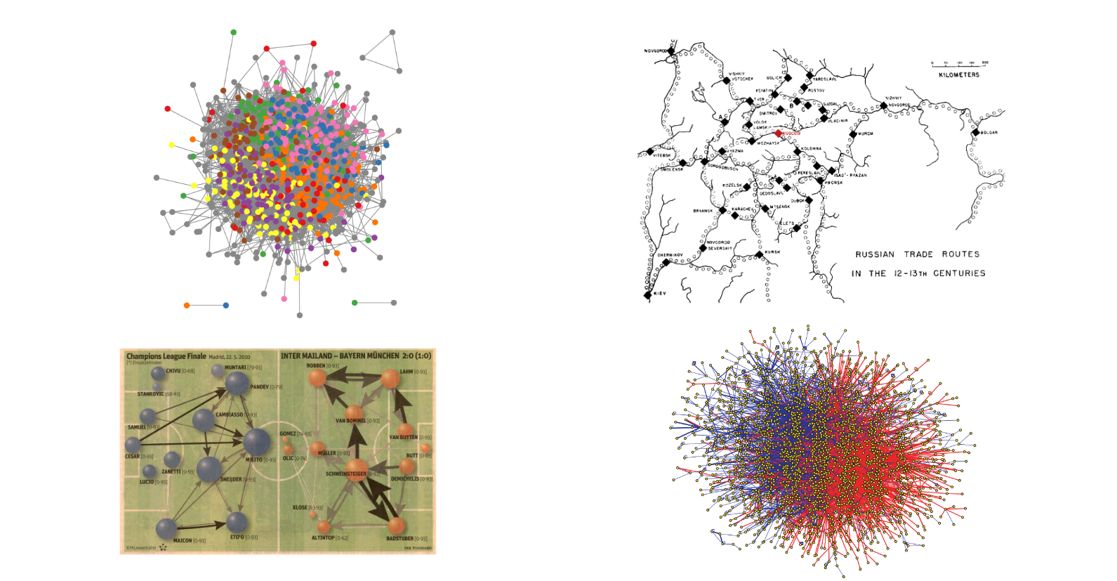
The image above illustrates four distinct network types, each from a unique domain:

• Top Left: Caltech Facebook Network
  This graph represents friendships between users in the Caltech Facebook network. Each node corresponds to an individual, and the edges depict social ties. By analyzing this network, we can identify patterns of social cohesion, community formation, and influential individuals within a university setting.

• Top Right: Historical Network of Russian Trade Routes (12th-13th Century)
  This network visualizes trade routes connecting major cities in medieval Russia. Nodes represent cities or trading posts, while edges reflect the trade pathways. Studying this historical network helps us understand economic dependencies and the geopolitical landscape of the time.

• Bottom Left: Soccer Match Pass Network
  This network shows passes between players in a soccer match, where nodes are the players and edges represent successful passes. Analyzing this network reveals team dynamics, key players, and overall passing strategy, offering insights into how teams organize and function during a game.

• Bottom Right: Protein-Protein Interaction Network
  This biological network visualizes interactions between proteins within an organism. Each node is a protein, and edges signify interactions between them. By examining this network, researchers can identify essential proteins and functional modules involved in cellular processes.

Analyzing networks allows us to achieve the following objectives:

• Description: Identifying and describing hidden community structures, clusters of closely related nodes, and general patterns in the network.
• Explanation: Providing insights into the underlying mechanisms or structural dependencies within the system (e.g., who influences whom in a social network, or how entities are interrelated in a technological network).
• Prediction: Forecasting future interactions or behaviors within the network, such as predicting the emergence of new relationships, or the likely behavior of system components based on current trends.

The process of analyzing networks typically follows a structured pipeline, as illustrated in the diagram below:

It begins with a clear problem statement, where the primary research question or challenge is identified. This is followed by the development of a theoretical framework, which provides the necessary background and context for understanding the network’s behavior. Based on this theory, hypotheses are formulated, offering testable predictions about the relationships and structures within the network.

Once the hypotheses are set, a research design is created, outlining the methods and tools that will be used to gather and analyze the data. The next step is data collection, where relevant network data is gathered from various sources, whether social, biological, or technological.

With the data in hand, the exploration and analysis phase begins. This step involves applying network analysis techniques to uncover hidden patterns, clusters, or dependencies within the network. Finally, the findings are brought together in the interpretation and presentation stage, where results are visualized and communicated to provide actionable insights or conclusions.

Challenges in Network Data

Analyzing network data presents several challenges:

• High Dimensionality: Networks can have millions of nodes and edges, making computational analysis difficult.
• Data Sparsity: Despite their large size, most nodes in a real-world network may not be directly connected.
• Dynamic Networks: Networks change over time, and algorithms need to account for these changes.
• Heterogeneous Networks: Some networks include multiple types of nodes and edges, adding complexity to their analysis.

Matrix Representation

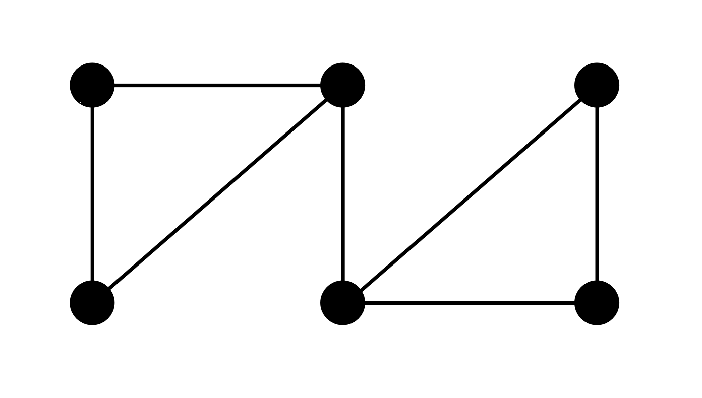
The adjacency matrix \(A \in \mathbb{R}^{n \times n}\) of a graph is defined as:

For undirected graphs, \(A\) is symmetric. For example, the adjacency matrix for a 6-node network is:

# Load necessary library
library(igraph)

# Define the adjacency matrix
adj_matrix <- matrix(c(0, 1, 1, 0, 0, 0,
                       1, 0, 1, 0, 0, 0,
                       1, 1, 0, 1, 0, 0,
                       0, 0, 1, 0, 1, 0,
                       0, 0, 0, 1, 0, 1,
                       0, 0, 0, 1, 1, 0),
                     nrow = 6, ncol = 6, byrow = TRUE)

# Create a graph object from the adjacency matrix
graph <- graph_from_adjacency_matrix(adj_matrix, mode = "undirected")

# Plot the graph
plot(graph, vertex.label = c("v1", "v2", "v3", "v4", "v5", "v6"),
     vertex.size = 30, 
     vertex.color = "lightblue", 
     edge.arrow.size = 0.5, 
     main = "Graph Representation of the Adjacency Matrix")
  

# Import necessary libraries
import networkx as nx
import matplotlib.pyplot as plt

# Define the adjacency matrix as a list of lists
adj_matrix = [
    [0, 1, 1, 0, 0, 0],
    [1, 0, 1, 0, 0, 0],
    [1, 1, 0, 1, 0, 0],
    [0, 0, 1, 0, 1, 0],
    [0, 0, 0, 1, 0, 1],
    [0, 0, 0, 1, 1, 0]
]

# Create a graph object from the adjacency matrix
G = nx.Graph(adj_matrix)

# Plot the graph
nx.draw(G, with_labels=True, node_color='lightblue', node_size=500, font_weight='bold')
plt.title('Graph Representation of the Adjacency Matrix')
plt.show()
  

Important Network Statistics

In social network analysis, several key statistics help us understand the structure and behavior of networks. These include degree, clustering coefficient, and path length, which we will explore in the context of social networks.

Degree of a Node

The degree of a node ( v_i ) is a fundamental statistic that refers to the number of direct connections (or edges) a person or entity has in a network. In social contexts, the degree of a node can represent the number of friends, colleagues, or connections an individual has.

For an undirected graph, where the connections are mutual (e.g., friendships), the degree is given by:

where ( A_{ij} ) is the element of the adjacency matrix that indicates whether there is a connection between nodes ( i ) and ( j ).

In a directed graph, such as Twitter where one user can follow another without mutual following, we distinguish between in-degree (the number of connections directed toward a node) and out-degree (the number of connections a node directs toward others):

• In-degree: \(k_i^{\text{in}} = \sum_j A_{ji}\) In a social context, this could represent the number of followers a person has on a social media platform.

• Out-degree: \(k_i^{\text{out}} = \sum_j A_{ij}\) This represents how many people a person follows or reaches out to, which might reflect their level of activity or influence in a network.

In social networks, a high degree often indicates centrality, suggesting that the individual is highly connected and potentially influential within their community.

Clustering Coefficient

The clustering coefficient ( C_i ) measures the degree to which a node’s neighbors are also connected to each other, reflecting the local cohesiveness of the network. In social networks, this can represent the tendency of a person’s friends to also be friends with each other. The clustering coefficient for a node ( v_i ) is calculated as:

where ( e_i ) is the number of edges between the neighbors of node ( v_i ), and ( k_i ) is the degree of the node.

In social network analysis, a high clustering coefficient might indicate tight-knit communities or groups where people know each other well (e.g., social cliques or circles). On the other hand, a low clustering coefficient might indicate a more dispersed network, where an individual connects with different, less interconnected groups. This is particularly relevant for analyzing phenomena like community detection or the spread of influence within social groups.

Path Length

Path length is a crucial statistic for understanding how information or influence spreads through social networks. The shortest path between two nodes, also known as the geodesic distance, is the minimum number of edges required to travel from one node to another. In social networks, this could represent how many intermediate connections are needed for information or influence to pass from one person to another.

Algorithms like Dijkstra’s or Floyd-Warshall are commonly used to compute the shortest path between nodes. The average path length ( L ) of a graph is given by:

where ( d(v_i, v_j) ) is the shortest distance between nodes ( v_i ) and ( v_j ), and ( n ) is the total number of nodes in the network.

In the context of social networks, the average path length indicates how quickly information can spread across the network. For example, in small-world networks, such as many social networks, the average path length is relatively short, reflecting the “six degrees of separation” phenomenon where most people can be connected in a few steps.

Multi-Hop Optimization Problem

In social network analysis, many problems require navigating through multiple hops between nodes. This is particularly relevant for multi-hop optimization problems, where the goal is to optimize paths or interactions over several steps, rather than just direct connections.

One common example of this is in viral marketing: to maximize the spread of information, product recommendations, or influence, one must consider not only the immediate neighbors but also the neighbors’ neighbors (and beyond). This multi-hop perspective helps in understanding how to strategically target individuals who can amplify a message through their connections, thereby optimizing the network spread.

Another important application of multi-hop optimization is in network resilience. When trying to improve the robustness of a social network (e.g., by ensuring that the network is still connected even if some individuals are removed), multi-hop paths provide alternative routes for information to flow, preventing bottlenecks and enhancing the system’s resilience.

Finally, in recommendation systems, multi-hop analysis can help in generating more personalized suggestions by exploring not just direct friends but also indirect connections, leveraging the broader network structure to make more accurate predictions.

By analyzing various aspects of networks—such as the degree of nodes, clustering coefficients, and path lengths—we gain critical insights into the structure and behavior of social networks. These analyses enable us to detect influential individuals, understand community structures, and predict the spread of information or behaviors.